In our Arabidopsis data set we have information on two time points (4 hrs and 14 hrs). In our previous differential expression example we only considered testing a single time point. However, we actually have lots more information than just this pairwise comparison. For example what about the relationship between the wild type between 4 and 14 hrs? Rather than conduct several tests of differential expression we can take an alternative approach and consider our expression data as a network.
Weighted gene co-expression network analysis (WGCNA) takes the view that there is more information to be gathered from expression data than a list of differentially expressed genes. Instead expression data is thought to be more completely represented by considering the relationships between measured transcripts. These relationships can be described by pairwise correlations between gene expression profiles. By examining all pairwise correlations between genes we can build a co-expression network where genes are represented by nodes, and the correlation of two gene’s expression profiles represents a connection or edge between them. If two genes are highly correlated then the edge between them is said to have a high weight.
WGCNA starts from the level of thousands of genes, identifies interesting gene modules (groups of genes with high similarity in expression profiles) and uses intra-modular connectivity and gene significance to identify key genes (referred to as eigengenes) in modules that could potentially be followed up in further validation studies. One strength of this approach is that the module definition does not make use of a priori defined gene sets i.e. genes annotated to the same pathway etc. Modules are defined solely on the expression profile data. Although it is possible to subsequently use the Gene Ontology to assess the biological plausibility of identified modules.
More information on WGCNA, including tutorials, can be found at here and you can read the original paper here.
Note: There are several steps in this analysis that will take a few minutes to run. I have included notes in bold when these steps are coming up. Currently, these steps are unavoidable to get a real experience of network analysis with RNA-Seq data. Feel free to grab a coffee or get on with something else while you wait!
We will begin by choosing our working directory
setwd("~/rna/deseq2_analysis/")
here we have set our working directory as the one that contains the count data. We will later change our directory so that we can right our outputs into a different folder.
If you haven’t already you will also need to load the DESeq2 package to be able to read in all the expression data.
library(DESeq2)
Next we can read the sample table with the same command as we have used previously:
sampleTable = read.table("sample.table")
Finally, we can read all the count data as before. Note that this time we want to read all the samples (not just the 14hr timepoint).
dcDESeqDataSet = DESeqDataSetFromHTSeqCount(sampleTable=sampleTable, directory = '.', design = formula(~strain))
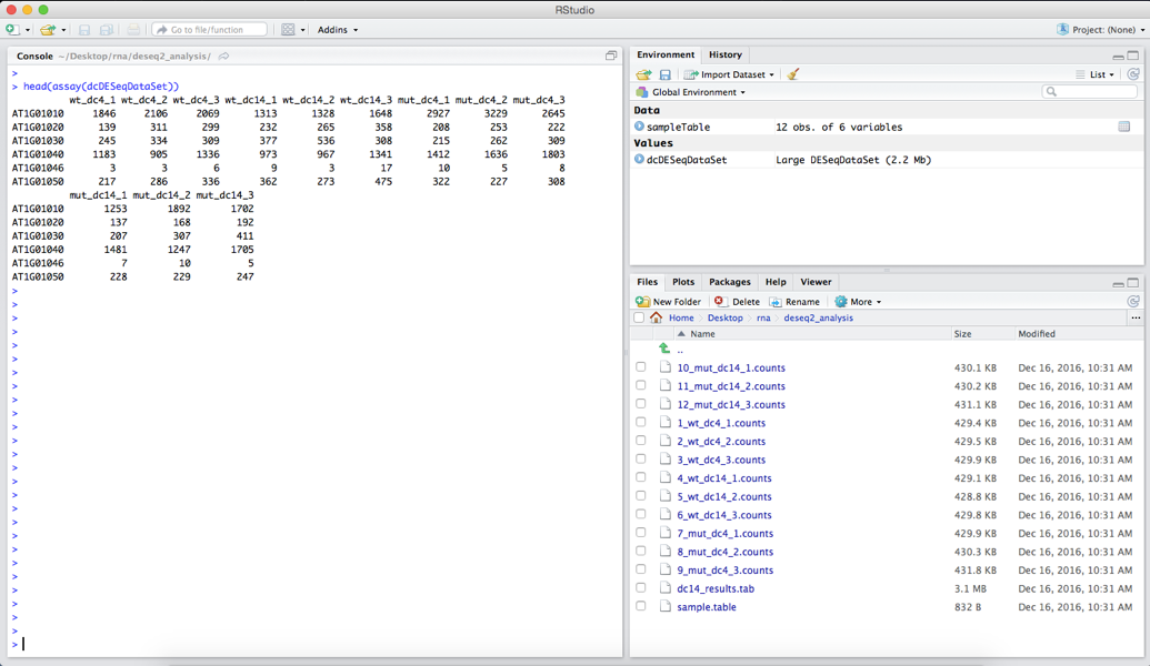
We can view the first few rows of these data with:
head(assay(dcDESeqDataSet))
your output should look like the image below:
We can see how many genes, each indicated by a single row, are in the dataset by using the command:
nrow(dcDESeqDataSet)
This tells us that we currently have 33,602 rows in our dataset.
Next we will want to apply some filtering and normalization to the data before we can use WGCNA. In the WGCNA guides and FAQs the authors recommend filtering rows with consistently low counts, which may represent noise and produce meaningless correlations. A filtering cutoff to remove rows with counts less than 10 in more than 90% of samples is suggested. This cutoff is somewhat subjective and will depend on the individual analysis and the underlying data. For this tutorial we will follow that suggestion and apply the filtering with the following commands:
keep = rowSums(counts(dcDESeqDataSet) > 10) >= 10
dcDESeqDataSet = dcDESeqDataSet[keep]
The first command produces a logical vector called ‘keep’ which stores TRUE if a gene have more than 10 counts (using counts()) in more than 10 samples (using rowSums()). The second command overrides our current dataset (dcDESeqDataSet) and only stores those rows that have a true value in the keep vector.
If we use the command:
head(assay(dcDESeqDataSet))
we can see that the gene ‘AT1G01046’ no loner appears in our dataset. This is because only one sample for this gene had more than 10 counts. Running:
nrow(dcDESeqDataSet)
shows us that we now have 17,202 genes in our dataset.
The authors of WGCNA also recommend that the count data be normalized before being analysed. Luckily for us DESeq2 implements a function called varianceStabilizingTransformation that will do exactly what we want. It is also worth mentioning that other normalisation methods can be applied, such as RPKM or FPKM, as long as all samples are treated the same way. Lets normalise our data using the command:
transformedData = varianceStabilizingTransformation(dcDESeqDataSet)
This command returns a DESeqTransform object that contains our transformed values that can be accessed with the assay() command. If you view the first few rows of the transformed data with:
head(assay(transformedData))
you will get the following output:
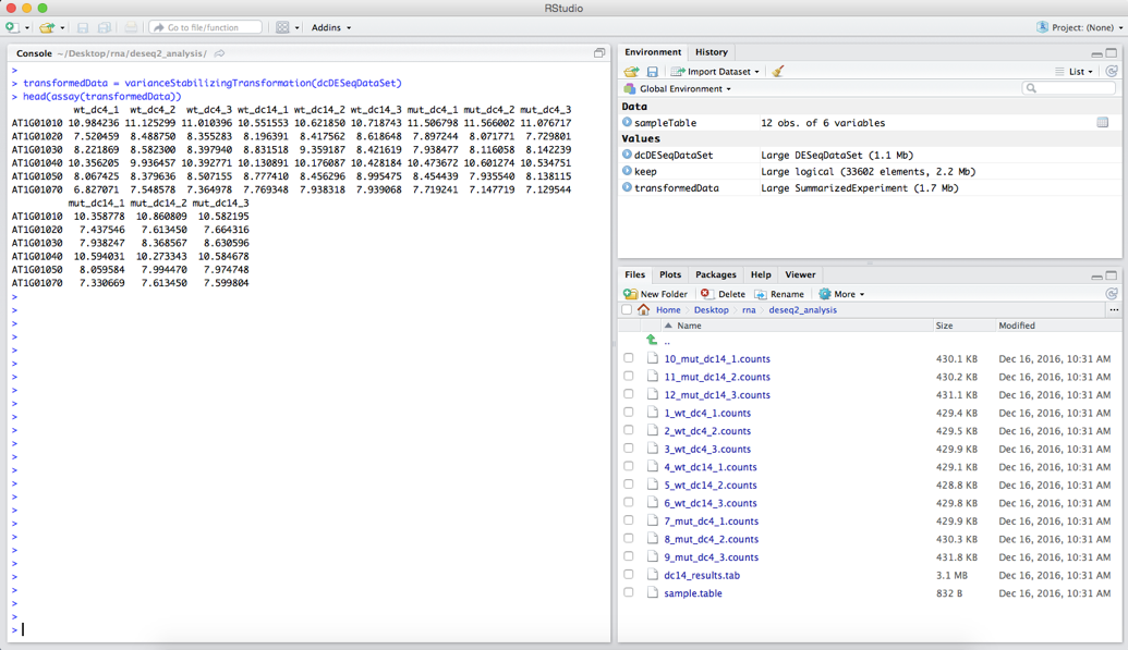
Notice that our values are no longer integer counts.
We are now ready to start using WGCNA. If you haven’t already we need to load the relevant package and set an option for reading text, which can be done with:
library(WGCNA)
options(stringsAsFactors = FALSE)
allowWGCNAThreads()
The first step in our task is to create a data frame of our expression data from ‘transfromedData’. Our data is currently organised as a matrix with column names representing treatments and row names representing genes. WGCNA wants its data where columns are genes and rows are treatments. We can create a relevant data frame using the command:
expr = as.data.frame(t(assay(transformedData)))
Here we create a data frame (as.data.frame) from our expression matrix (assay(transformedData)) and transpose the matrix using the command t(). Our data should now be ready to be used with WGCNA.
Our first step will be to check the quality of our input data. We want to ensure that we don’t have any samples with missing values:
gsg = goodSamplesGenes(expr, verbose = 3)
The returned list object ‘gsg’ contains 3 values; (i) a list of good genes, (ii) a list of good samples and (iii) a logical value about whether all genes are OK. We can check this by typing:
gsg$allOK
This returns ‘TRUE’ indicating that our data does not contain any missing values. We should expect this test to return ‘TRUE’ as we already used some of DESeq2’s functions to filter our data based on the recommendations by WGCNA’s authors.
Now that we are satisfied that are data is suitable for analysis lets start our network construction and module detection steps. It should be noted that WGCNA has several methods for network construction and module detection. Tutorials for these approaches are available. In this workshop we are going to follow the automatic, one-step method for network construction and module detection.
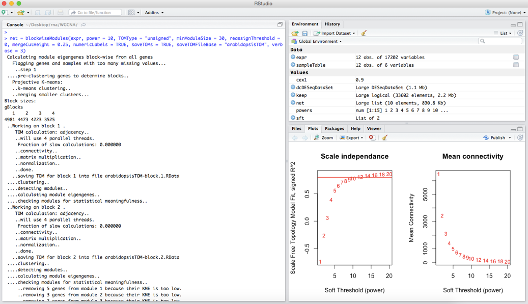
Our first step is to pick a ‘soft thresholding power’. This power is applied to co-expression similarities, in our case correlations in expression profiles, to calculate adjacency i.e. which genes are connected in our network. The authors of WGCNA suggest that users can use the scale free topology of the graph i.e. numbers of highly connected and lowly connected nodes, to help choose a relevant soft thresholding power. WGCNA provides the function pickSoftThreshold to help the user with this task. We will start this step with:
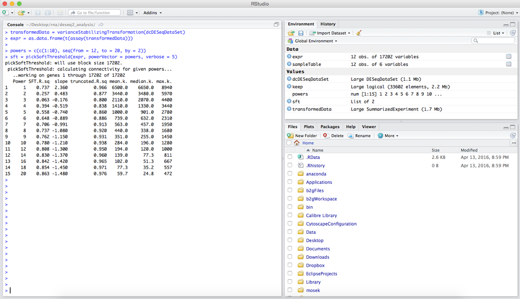
powers = c(c(1:10), seq(from = 12, to = 20, by = 2))
sft = pickSoftThreshold(expr, powerVector = powers, verbose = 5)
First we create a vector or powers that just contains the numbers 1 to 10 and then 12 to 20 going up by 2 (seq()). These are the soft thresholding powers that we want to try. The second command runs the pickSoftThreshold function of WGCNA that will help us in deciding a thresholding power. This command may take a few minutes to run, and when it finishes you should see some information printed to the console.
Although all the necessary information to pick a soft thresholding power is output here, it is much easier to interpret when we plot these values. The following commands will produce two plots:
sizeGrWindow(9, 5)
par(mfrow = c(1, 2))
cex1 = 0.9
plot(sft$fitIndices[,1], -sign(sft$fitIndices[,3])*sft$fitIndices[,2], xlab="Soft Threshold (power)", ylab = "scale Free Topology Model Fit, signed R^2", type = "n", main = paste("Scale independence"))
text(sft$fitIndices[,1], -sign(sft$fitIndices[,3])*sft$fitIndices[,2], labels = powers, cex = cex1, col = "red")
abline(h = 0.8, col = "red")
plot(sft$fitIndices[,1], sft$fitIndices[,5], xlab = "Soft Threshold (power)", ylab = "Mean Connectivity", type = "n", main = paste("Mean connectivity"))
text(sft$fitIndices[,1], sft$fitIndices[,5], labels=powers, cex = cex1, col="red")
The output of these commands should look something like:
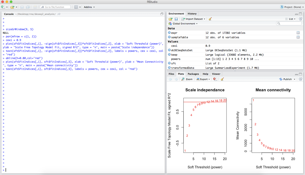
We want to choose the lowest power for which the scale-free topology fit index curve flattens out upon reaching a high value – where we have drawn a line at R-squared = 0.8. In this case we will pick a soft thresholding power of 10.
We will shortly start to save data from our network analysis so we will first move into a WGCNA folder, in which we can save some output:
setwd("~/rna_tutorial/WGCNA/")
Now we are ready to construct the gene network and identify modules. This can be done with a simple functions call:
net = blockwiseModules(expr, power = 10, TOMType = "unsigned", minModuleSize = 30, reassignThreshold = 0, mergeCutHeight = 0.25, numericLabels = TRUE, saveTOMs = TRUE, saveTOMFileBase = "arabidopsisTOM", verbose = 3)
This command contains a lot of options:
expr – our expression datapower – our choice of soft thresholding powerTOMType – the type of network. In a signed network correlations will range from -1 to 1. In an unsigned network correlations will range from 0 to 1 where positive and negative correlations will be treated identically.minModuleSize – the size in number of genes of the smallest allowed clusterreassignThreshold – a p-value threshold for reassigning genes between modules – a value of 0 means that genes cannot be reassigned between modules.mergeCutHeight – dendrogram cut height for module mergingnumericLabels – module names are integers rather than colour namessaveTOMs – should the consensus topological overlap matrices (TOMs) be saved during the analysissaveTOMFileBase – the name of the file to save the TOMsverbose – how much information to print to the consoleYou should note that the function blockwiseModules has a vast array of options that you can tune and change to suit your analysis. You can view the whole range of options with the command:
?blockwiseModules
The options I have set in this example are based on the WGCNA tutorial but you should change these based on your own data and analysis. This command will take a few minutes to run and the progress will be printed to the screen.
Next we can take a quick look at the number of modules identified and their size with the command
table(net$colors)
We can see that there are 25 clusters identified (NB the 0 cluster is not really a cluster but a group containing genes that couldn’t be assigned to a cluster). These clusters range in size from 3,717 genes to only 36 genes.
We can also view the dendrogram (tree) that was used to define these clusters:
sizeGrWindow(12, 9)
mergedColors = labels2colors(net$colors)
plotDendroAndColors(net$dendrograms[[1]], mergedColors[net$blockGenes[[1]]], "Module colors", dendroLabels = FALSE, hang = 0.03, addGuide = TRUE, guideHang = 0.05)
This produces the image:
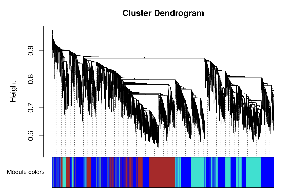
The image shows the dendrogram that was built from our co-expression network. We can then see at the bottom of the image, the clusters to which the genes were assigned. Here the clusters are now represented as colours. We can see that the blue, red and turquoise clusters are large and contain many genes.
One useful function here would be to write the cluster/module membership to a file that can be used in other software or online tools. This can be achieved with two easy commands:
moduleAssignment = data.frame(GeneName = names(expr), Assignment = net$colors)
write.table(moduleAssignment, file = "Arabidopsis_clusters.txt", row.names = FALSE, quote = FALSE)
In the first command we make a new data frame with two columns. In the first column contains all of the genes in the analysis and the second column contains the module assignment for that gene as an integer ID. The second command uses the write.table() function to write the information to a file called ‘Arabidopsis_clusters.txt’.
It is a common analysis to test for enrichment of GO terms in clusters in order to determine their function. This can be done with several online tools such as DAVID, AmiGO and the R tools described in the previous section.
As an example lets look for GO enrichment in a single module in our data. First we create a named vector that stores all the genes in the network.
allGenes = rep(0, length(names(expr)))
names(allGenes) = names(expr)
This is a named vector that stores all the genes in the network where each gene has a corresponding value of 0 (rep()). Next we want to select a single module from our network. In this example we will choose the red module.
module = "red"
inModule = is.finite(match(labels2colors(net$color), module))
modGenes = names(expr[inModule])
Here, we create a vector that stores all the genes in the red module. Note the use of the match function to get all the genes where the colour of the module is listed as red. Next we give all the genes in the red module a value of 1 in our allGenes vector:
allGenes[modGenes] = 1
Now we have prepared our named vector we can test for GO enrichment as we did in the previous section. We start by creating a function to select all the genes in the red module (those that have a value of 1) from a vector:
selGenes = function(allGenes) { return(allGenes == 1) }
Next, we create the GOdata object using our new allGenes vector and our new function to select module genes:
GOdata = new("topGOdata", ontology = "BP", allGenes = allGenes, geneSel = selGenes, description = "GO analysis of WGCNA module", annot = annFUN.org, mapping = "org.At.tair.db")
We run the Fisher’s exact test to look for enrichment:
resultFisher = runTest(GOdata, algorithm = "classic", statistic = "fisher")
Create a results table:
resultsTable = GenTable(GOdata, classicFisher = resultFisher, orderBy = "classicFisher", topNodes = length(usedGO(object = GOdata)))
Adjust for a false discovery rate:
adjusted = p.adjust(score(resultFisher), method="BH")
adjustedP = data.frame(GO.ID = names(adjusted), correctedFisher = adjusted)
resultsTable = merge(resultsTable, adjustedP, by.x = "GO.ID", by.y = "GO.ID")
Reorder the results:
resultTable = resultTable[order(resultTable$correctedFisher), ]
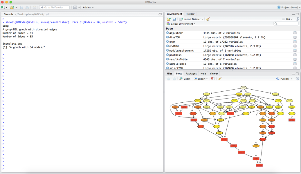
And finally visualize the GO:
showSigOfNodes(GOdata, score(resultFisher), firstSigNodes = 10, useInfo = "def")
The results suggest that the red module is associated with metabolism and photosynthesis in the presence of light. The output will look like:
WGCNA provides some methods for visualising the network. One visualisation method is to create a heatmap from the weighted network. In this image each row and column of the heatmap correspond to a single gene. The heatmap can depict adjacencies or topological overlaps, with light colours denoting low adjacency (overlap) and darker colours higher adjacency (overlap). In addition, the gene dendrograms and module colours are plotted along the top and left side of the heatmap. It should be noted that this approach can only be taken if the network was built using a 1-step approach, as we did in this tutorial. You can produce a heatmap with the following code:
moduleLabels = net$color
moduleColours = labels2colors(net$color)
geneTree = net$dendrogram[[1]]
nGenes = ncol(expr)
nSamples = nrow(expr)
First we just set up some useful variables that contain the module labels, colours, the gene tree and the number of genes and samples in our data. Next we recalculate the topological overlap matrix. Please note that this next command may take a while to run (>10 mins). I’d get a coffee or have a break while this is running!
dissTOM = 1- TOMsimilarityFromExpr(expr, power=10)
As the plotting can take a long time to run we will actually only plot a subset of genes. So next we select only 400 genes from the data set. By setting a seed value we can ensure that our random selection will be repeatable. We select these genes from the topological overlap matrix, create a new gene tree from these genes and then select the relevant modules that are represented by these genes.
set.seed(10)
nSelect = 400
select = sample(nGenes, size = nSelect)
selectTOM = dissTOM[select, select]

selectTree = hclust(as.dist(selectTOM), method = "average")
selectColours = moduleColours[select]
In the next command we next transform the matrix with a power to make moderately strong connections more visible in the heatmap. Then we set the diagonal of the plot to NA, which just makes the plot look a little nicer.
plotDiss = selectTOM^7
diag(plotDiss) = NA
Finally, we create a plot and then plot the heatmap, where we provide the matrix, gene dendrogram and module assignments.
sizeGrWindow(9, 9)
TOMplot(plotDiss, selectTree, selectColours, main = "Network heatmap plot, 400 genes")
The output of these commands should look something like:
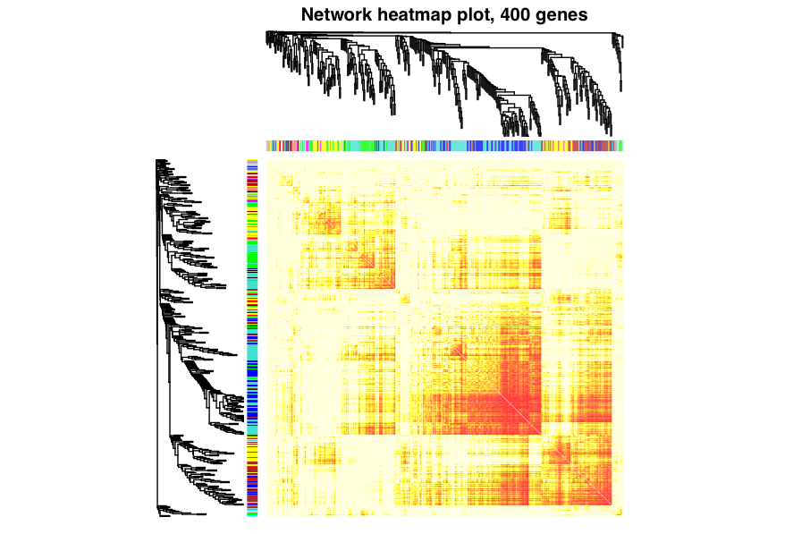
The heatmap depicts the topological overlap matrix among 400 selected genes. Light colors show low overlap (weak/no connections) and darker colours represent higher overlap (many/highly connected). Blocks of colour next to the dendrograms show the module membership for the genes. Blocks of darker colours on the diagonal are the modules and correlated with the module colours on the x and y axes. The dendrogram of the genes in the analysis are also shown on the x and y axes.
Cytoscape is a network viewer that is often used to create publication quality figures of networks. In addition, Cytoscape also has a variety of plugins that can be used for additional network analysis. In this section we will write out some module information that can be used by Cytoscape. Cytoscape requires an edge file and a node file, allowing the user to specify for example link weights and node colours.
We start by again recalculating the topological overlap matrix:
TOM = TOMsimilarityFromExpr(expr, power = 10)
Next, we will pick a module that we want to export and create a logical vector of all the genes in the module and then select those genes from our expression data:
module = "red"
inModule = is.finite(match(moduleColours, module))
modGenes = names(expr[inModule])
Next, we select a subset of the topological overlap matrix that contains information for our module of interest:
modTOM = TOM[inModule, inModule]
Finally, we use the function exportNetworkToCytoscape to write the files that can be used to load a network in cytoscape:
cyt = exportNetworkToCytoscape(modTOM, edgeFile = paste("CytoscapeInput-edges-", paste(module, collapse="-"), ".txt", sep=""), nodeFile = paste("CytoscapeInput-nodes-", paste(module, collapse="-"), ".txt", sep=""), weighted = TRUE, threshold = 0.2, nodeNames = modGenes, nodeAttr = moduleColours[inModule])
There are some useful parameters in this function call:
weighted – TRUE specifies that the network has edge weightsthreshold – is used to specify a minimum correlation cutoff to specify an edgeYou can view these files with less to see there format. Note, that if instead of storing a single module name in the variable ‘module’ we could have made this a vector and stored multiple module names. The rest of the code would have then written edge and node files for each module.
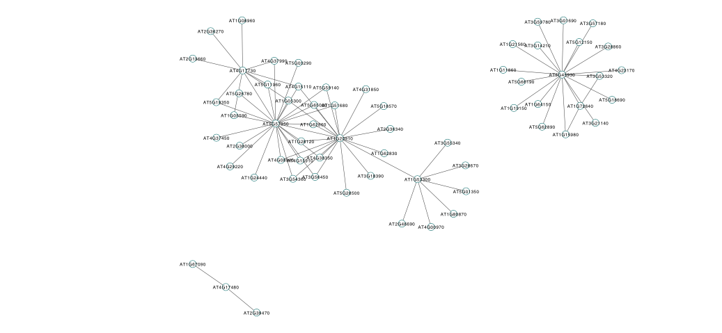
If you were to view these files in Cytoscape you could make an image such as:
You should now have gained some experience of network analysis using Weighted Gene Coexpression Network Analysis (WGCNA). We have