In the previous section you produced a list of differentially expressed genes in A. thaliana using DE-Seq2. The next step in our analysis will be to identify Gene Ontology (GO) terms that are enriched in the list of differentially expressed genes. The GO provides a controlled vocabulary of terms for describing gene product characteristics and gene product annotation data. The GO can be found at geneontology.org.
We will carry out our GO enrichment analysis using R and the package topGO. The topGO package is designed to facilitate semi-automated enrichment analysis for GO terms. The process consists of input of normalized gene expression measurements, gene-wise correlation or differential expression analysis of GO terms, interpretation and visualization of the results.
Still in RStudio load the topGO package with
library(topGO)
As we have all of our differential expression data in a DESeq2 object, we can load the list of differentially expressed genes directly with:
data = results(dc14DESeqDataSet)
We can see the number of genes in the data set with the command:
length(row.names(data))
One potential problem is that some genes have no expression data and should not be included in the analysis because we cannot determine whether they are not expressed or are missed because of the sequencing procedure. To remove the genes with no expression data we can use:
data = data[complete.cases(data), ]
This command selects the rows from data that are complete cases i.e. each field in the row has information (not NA). We then assign the selected rows to the data object. We can see now that the new data object has a different number of rows.
length(row.names(data))
Now we need to prepare the data for use with the topGO package. We can see from the topGO user guide (see topGO bioconductor page)that we need (i) a named vector of gene names and scores (i.e. p-values for differential expression), (ii) a function to select significant genes based on score and (iii) a mapping between gene identifiers and GO terms.
(i) To define a named vector of gene names and scores (p-values from DE-Seq2) we use the commands
genes = data$padj
names(genes) = row.names(data)
These commands create a vector named genes that contains the adjusted p-values from DE-Seq2. The names() command is then used to set the names of the genes associated with the p-values.
(ii) Next we need to declare a function that will be used to select those genes that are interesting for the analysis i.e. significantly differentially expressed genes
deGenes = function(genes) { return(genes < 0.05) }
Here we create a function called deGenes(). We define a function using the function command and specify that it accepts as input the genes vector of p-values. We then specify that we want to return rows from the genes vector where the value is less than 0.05.
(iii) The final step for preparing the GO enrichment analysis is to create a mapping between GO terms and genes. Fortunately, R has several built in GO databases that include mappings between GO terms and genes. We can load a A. thaliana specific database with the command:
library(org.At.tair.db)
Now we are ready to start our GO enrichment analysis. The first step is to create a GO data object
GOdata = new("topGOdata", ontology = "BP", allGenes = genes, geneSel = deGenes, description = "GO analysis for RNA-Seq workshop", annot = annFUN.org, mapping = "org.At.tair.db")
This lengthy command requires some description:
ontology = “BP” – which ontology of the gene ontology should be used for the analysis. Here we are using the Biological Process ontology.allGenes = genes – Specifiy the named vector containing all the genes in the enrichment analysis. We specify the genes named vector created earlier.geneSel = deGenes – The function that should be used to select the genes of interest for the enrichment analysis. We used the deGenes function that selects genes with a p-value less than 0.05.description – a text description of the analysis.annot = annFUN.gene2GO – Specify the gene to GO term mappings function. Here we using the built in organism databases.mapping = “org.At.tair.db” – As we are using one of the built in databases we need to specify the specific organism database. Here we specify “org.At.tair.db” which is the A. thaliana database.Now we can run Fisher’s exact test to identify GO term enrichment.
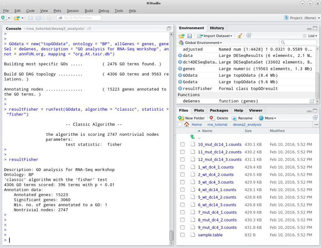
resultFisher = runTest(GOdata, algorithm = "classic", statistic = "fisher")
Here we have run the Fisher’s exact test using the ‘classic’ algorithm on our GO data object and stored the result in the object resultFisher. We can see some summary statistics about our analysis with:
resultFisher
Now it would be useful to export the data in a readable format i.e. a table. We can use topGO’s GenTable() function to generate a data frame with all the information for a table.
resultTable = GenTable(GOdata, classicFisher = resultFisher, orderBy = "classicFisher", topNodes = length(usedGO(object = GOdata)))
This is another lengthy command in need of further description:
classicFisher = resultFisher – The table can display more than one result and topGO has many different tests for enrichment. Here we specify that we have used the classicFisher method and point the method to the appropriate object.orderBy = “classicFisher” – We can order the table by several different values/columns and here we order the table by the p-value from the classicFisher analysis.topNodes = length(usedGO(object = GOdata)) – This command specifies the number of GO terms to be reported in the table. The length and usedGO functions determine the number of GO terms used in the analysis so that the table reports all GO terms rather than an arbitrary number.In this analysis we have conducted many Fisher’s exact tests, to correct for type 1 errors (i.e. false positives) we might want to apply some false discovery rate (FDR) correction. We can apply some FDR correction using the p.adjust() method in R.
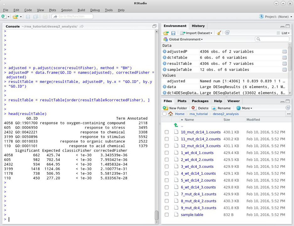
adjusted = p.adjust(score(resultFisher), method = "BH")
adjustedP = data.frame(GO.ID = names(adjusted), correctedFisher = adjusted)
resultTable = merge(resultTable, adjustedP, by.x = "GO.ID", by.y = "GO.ID")
The p.adjust method takes the scores (p-values) from the resultFisher object and applies FDR correction using the method of Benjamini and Hochberg (BH). The second command converts the named vector returned by p.adjust into an R data frame where the column GO.ID stores GO terms and correctedFisher stores the adjusted p-values. Finally, we merge our new data frame with the results table (resultTable) on the GO term column. The result is a new resultTable data frame with an additional column for corrected p-value.
After p-value correction we will want to sort our results table again – this time sorting on the adjusted p-value.
resultTable = resultTable[order(resultTable$correctedFisher), ]
head(resultTable)
Now we are ready to write the results to a file. To write the results for all the GO terms in the analysis we can use
write.table(resultTable, file = "all_enrichment.txt", quote = F, sep = "\t", row.names = F)
In this command we specify several formatting options:
resultTable – the data frame storing the results of the GO enrichment analysisfile = “all_enrichment.txt” – The file namequote = F – Do not put quote around the text outputsep = “\t” – Create a tab separated filerow.names = F – Rows are numbered in the data frame setting row.names = FALSE stops R from writing row numbers in the output fileTo write only the terms that are significant after FDR correction we can use
write.table(resultTable[resultTable$correctedFisher < 0.05, ], file = "signif_enrichment.txt", quote = F, sep = "\t", row.names = F)
In the write.table function we specify several formatting options:
resultTable[resultTable$correctedFisher < 0.05, ] – selecting only rows with a correct-ed Fisher value of less than 0.05file = “signif_enrichment.txt” – The file namequote = F – Do not put quote around the text outputsep = “\t” – Create a tab separated filerow.names = F – Rows are numbered in the data frame setting row.names = FALSE stops R from writing row numbers in the output fileA useful way of looking at the results of the analysis is to investigate how the significant GO terms are distributed over the GO graph. We can use topGO to visualise the subgraphs induced by the most significant GO terms stored in the resultFisher object.
To view the subgraph in the current graphics device we can use the command:
showSigOfNodes(GOdata, score(resultFisher), firstSigNodes = 10, useInfo = "def")
Here we pass several arguments to the function:
GOdata – our GO data objectscore(resultFisher) – the p-value scores from the enrichment analysis – this is a named vectorfirstSigNodes – the number of top scoring GO terms to use in the visualisationuseInfo – the additional information to include in the plot. Using ‘def’ prints the GO term definition in the plot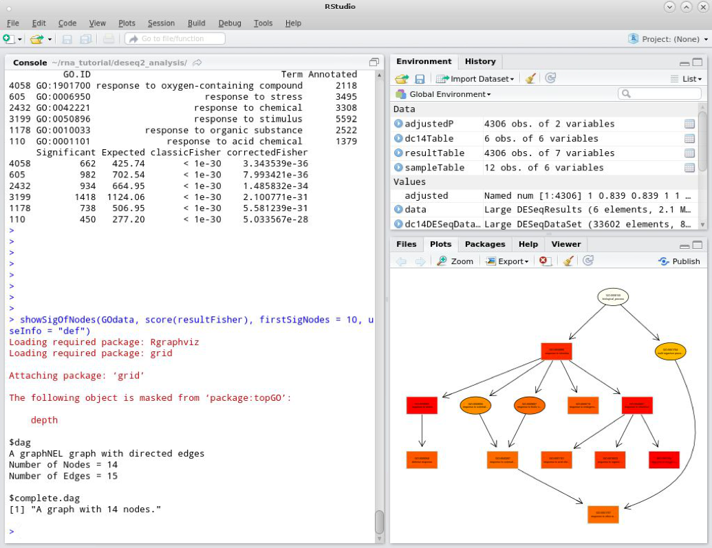
One issue with this visualisation is that it uses the raw p-values for the plot. After multiple testing correction it might be that some significant raw p-values are not significant after correction. Therefore it might be best to use the corrected p-values in this plot. We can do this easily by making a named vector of corrected p-values to replace score(resultFisher) in the above example. To create the new named vector we can use the following commands:
correctedFisher = resultTable$correctedFisher
names(correctedFisher) = resultTable$GO.ID
These commands create a new vector called correctedFisher that stores our corrected p-values. We then use the names() function to assign names to the vector. Next we can re-draw our GO visualisation.
showSigOfNodes(GOdata, correctedFisher, firstSigNodes = 10, useInfo = "def")
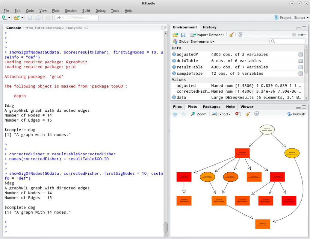
As you can see the visualisation is unchanged from the previous version though this will not always be the case and will depend on the data set.
You can save these visualisations directly from the R graphics window.
In some cases you might not want to open a visualisation in a graphics window. For example you might be creating many visualisations in a script and having to save each image manually would be very time consuming. Instead we can output images directly to a file.
One method of writing images to a file it to use the pdf() function:
pdf(file = "go_structure.pdf")
showSigOfNodes(GOdata, correctedFisher, firstSigNodes = 10, useInfo = "def")
dev.off()
Here we open a PDF file/graphics device named ‘go_structure.pdf’. We then plot the figure as normal. Finally we use dev.off() to close the PDF graphics device. This is very important to ensure that the plot is completed and the file is saved.
An alternative approach to plotting the GO subgraph to a file is to use the printGraph() function provided by topGO:
printGraph(GOdata, resultFisher, firstSigNodes = 10, fn.prefix = "go_structure", useInfo = "def", pdfSW = TRUE)
This command will produce the file ‘go_structure_classic_10_def.pdf’ in your working directory.
You should now have gained some experience of Gene Ontology enrichment analysis for differentially expressed genes. We have
topGO is only one of many available tools for GO enrichment analysis. Some popular alternatives are: