DESeq2 is a software package that takes gene expression data such as we have just produced using htseq-count. It tests for differential expression of each gene based on a model using the negative binomial distribution. You can read more about DESeq2 at bioconductor and in the original paper.
DESeq2 requires you to enter a few commands using R to get your results. If you don’t understand the R commands exactly, you can review the DESeq2 manual.
Our starting point for this analysis will be count files produced by htseq-count. These files are prep-prepared but have exactly the same format as you saw in the previous section. First lets navigate to the correct folder
cd ~/rna_tutorial/deseq2_analysis
We can view the files in the directory
ls -lh
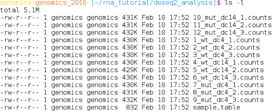
There are 12 count files, one for each plant. The format of the file names is:
There is also a file called ‘sample.table’ that we will view in R.
Start R-studio by double clicking the R-studio icon on the Desktop. The window that opens should look something like:
On the left hand side is the console. This is where we will input the rest of the workshop commands. On the right hand side is the environment, which will give us information about the variables we will create and use. Below the environment is the files tab, which shows the directory structure of the machine. There are other tabs here, such as the plots tab, that are useful and can help you set up an effective development environment.
In the console tab lets type our first command to set the current working directory
setwd("~/rna_tutorial/deseq2_analysis")
We will us number of R packages to analyse and visualise our data. You can load them all before we start. If you leave your R session, you can save your work in a workspace but you will need to reload these packages to resume your analysis.
library(DESeq2)
library(ggplot2)
library("genefilter")
library("RColorBrewer")
library("pheatmap")
now let’s look at the ‘sample.table’ file
read.table("sample.table", header=TRUE)
The output will look something like
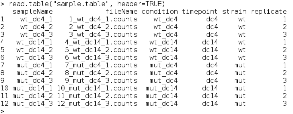
The table is in the precise format that DESeq2 understands. The first 2 columns ‘sampleName’ and ‘fileName’ are required - the other columns can be any factors that you want them to be, and you can use them to tell DESeq2 what to include in the analysis.
We will need to use this table again so save it in a variable sampleTable
sampleTable = read.table("sample.table")
One thing we have to be careful of is that DESeq2 knows the order you want to apply to the conditions or factors in your experiment - so for example in our experiment it would be normal to compare the mutant to the wild type. So a positive change in an expression level for a gene means that the gene has been upregulated in the mutant and a negative change implies downregulation. That would fit our intuitive understanding of up and downregulated in our context.
In R, by default the factors are ordered alphabetically so if we type:
levels(sampleTable$strain)
We see that the mutant comes before the wild type. Intuitively we want a positive fold change in gene expression to mean that it is higher in the mutant. To tell DESeq2 that we want to always compare the mutant with the wild type enter the command:
sampleTable$strain = relevel(sampleTable$strain,"wt")
Re-running the levels command shows us that we have re-ordered our conditions
levels(sampleTable$strain)
We should do this for all the factors, but we are only using strain for now.
Let simplify the experiment for now.
dc14Table = sampleTable[sampleTable$timepoint == 'dc14',]
dc14Table
Which gives:
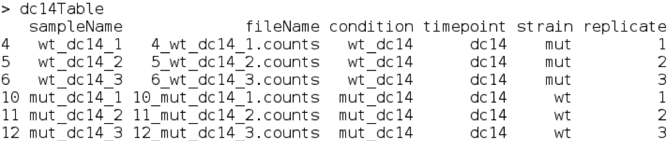
Now we have selected just one time-point and we can simply compare the three mutant samples to the 3 wildtype samples. This will form the basis of the most simple type of differential expression analysis.