So far we have counted the number of reads for each gene in each sample and get it into a form that DESeq2 can analyse, displayed a heatmap (with clustering) of the top 50 most variable genes and created a PCA plot of our samples. We are now ready to find up and downregulated genes.
Note: that we use the raw counts of the gene expression rather than the log transform which we used for visualisation.
To run the DESeq2 analysis:
dc14DESeqDataSet = DESeq(dc14DESeqDataSet)
You’ll see some text representing the progress of the analysis and once it has finished you can see the format of the results:
results(dc14DESeqDataSet)
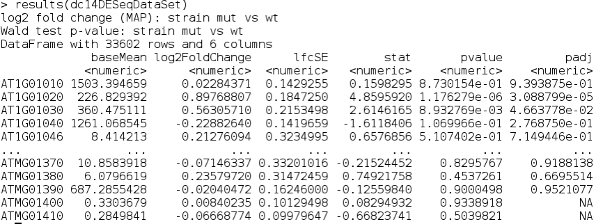
You can also get a description of the columns:
mcols(results(dc14DESeqDataSet),use.names=T)
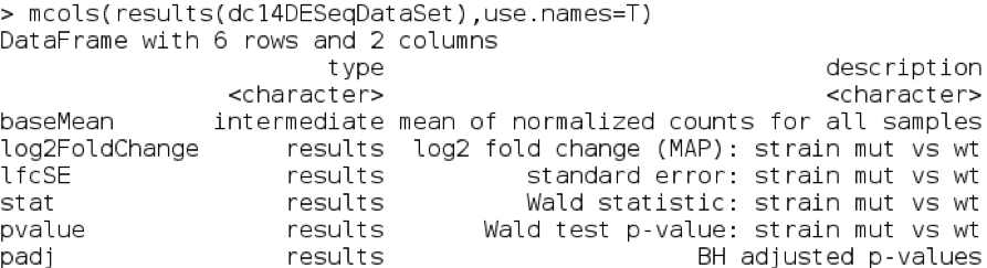
The columns we are most interested in (unless you are a statistician) are:
Let’s check the 10 most significantly upregulated genes and see whether the calculations look plausible.
First lets extract the top 10 differentially expressed genes (ranked by padj values)
topUpregGenes = head(order(results(dc14DESeqDataSet)$padj),n=10)
results(dc14DESeqDataSet)[topUpregGenes,]
If we look at AT5G47390 we can see that the log2FoldChange tells us that the gene seems to be upregulated in the mutant strain and the padj value shows us that this change is highly significant. As a sanity check we can look at the raw count numbers these genes:
assay(dc14DESeqDataSet)[topUpregGenes,]
The counts confirm the identified differential expression with the mutant strains showing many more counts in AT5G47390 than in the wild-type strains.
We can also use an MA Plot visualize all the results. This plots the log ratio (M) on the x axis and the average expression (A) on the y axis.
plotMA(dc14DESeqDataSet,ylim=c(-2.5,2.5))
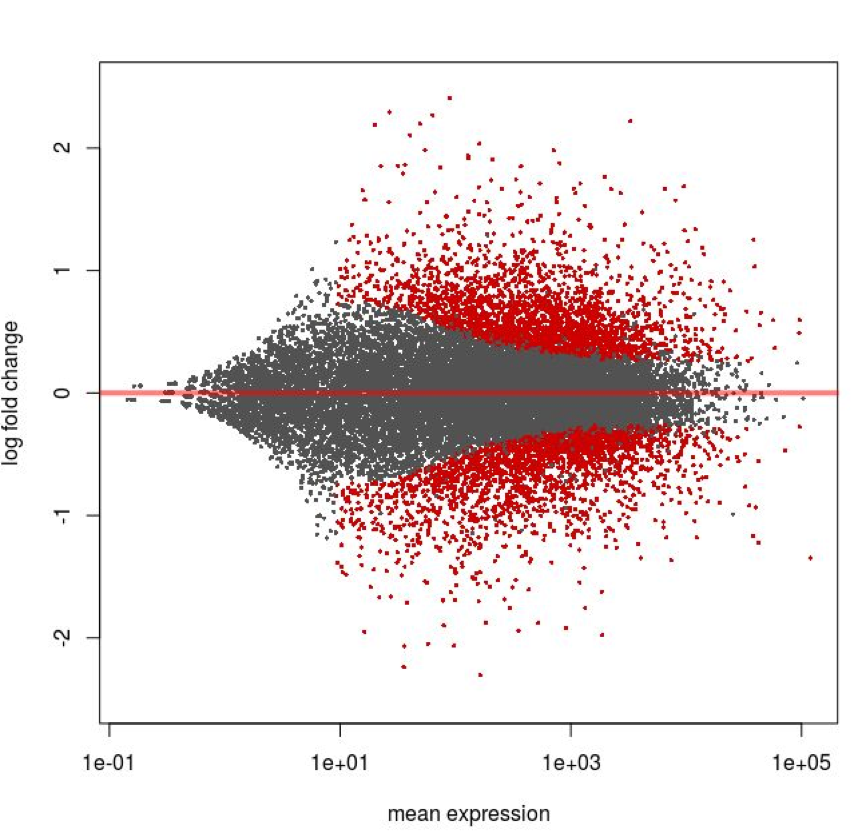
This plot shows one point for each gene - if DESeq2 considers the gene to be significantly up or down regulated it is shown in red, otherwise in grey. The curved boundary between red and grey shows that as the expression level of the gene increases DESeq2 can call genes with lower fold change ratios.
A large number of genes have been identified as being differentially regulated; this is consistent with the large difference in phenotypic response of the two strains.
To create files containing all statistically significantly up and down-regulated (by 2 fold) genes we use the which() command to select them
downregGenes = which(results(dc14DESeqDataSet)$log2FoldChange < -1)
upregGenes = which(results(dc14DESeqDataSet)$log2FoldChange > 1)
Remember here that a 2 fold change in expression is represented by a log2 fold change of 1.
Next, we extract all the genes that show significant differential expression using a padj cutoff of 0.05.
sigGenes = which(results(dc14DESeqDataSet)$padj < 0.05)
Finally, we write the intersection (appears in both) of significantly differentially expressed genes with those that are up and down regulated. These files will be useful for downstream analysis programs or for making tables for publications.
write.table (file='downreg.tab', results(dc14DESeqDataSet) [intersect(downregGenes, sigGenes ),])
write.table (file='upreg.tab', results(dc14DESeqDataSet) [intersect(upregGenes, sigGenes ),])
You should have some appreciation of the process and challenges of analysing RNA-seq data for differentially expressed genes. To recap the process we followed was: