From the heatmap we generated above we can see that our samples are clustered by strains - the three wild type samples, and the three mutant samples are more similar to each other than to samples from the other group. This is good for our experiment because it suggests that the signal that we are interested in is larger than biological noise in our samples.
Another way to visualise this is to perform a principle component analysis (PCA)
plotPCA(dc14DESeqDataSet.rld , intgroup = c('strain'))
We can label the points (and change the axis limits to allow for them)
plotPCA(dc14DESeqDataSet.rld , intgroup = c('strain'))+ geom_text(aes(label=colnames(dc14DESeqDataSet.rld)),hjust=1.2) +xlim(-15,10) + ylim(-5,5)
The output should look something like:
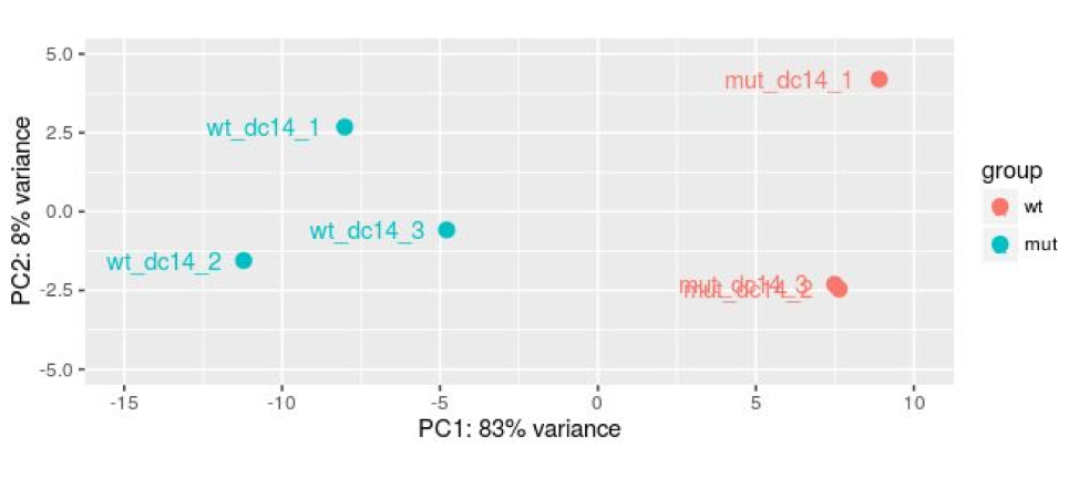
plotPCA identifies the strongest principle components in the dataset and plots them, the numbers themselves are not meaningful. In the graph above the first principle component (PC) accounts for 83% of the variation in the samples (this is unusually high) and we have good separation of our groups on this component. The second component accounts for 8% of the variation and we do not see any separation of our groups.