Next, we load the htseq-count data from the .counts files
dc14DESeqDataSet = DESeqDataSetFromHTSeqCount(sampleTable=dc14Table, directory='.', design=formula(~ strain))
This loads the count data for all the samples in dc14Table - DESeq2 uses the information in the table to associate each sample to the correct count file. We are also telling DESeq2 that we intent to use the strain column to group samples for comparison.
To see the results type:
assay(dc14DESeqDataSet)
or to show just a few rows:
head(assay(dc14DESeqDataSet))
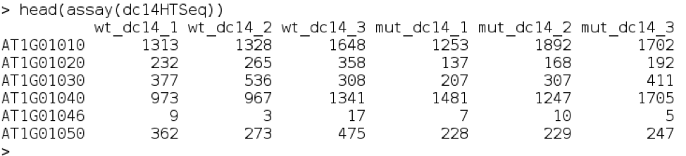
You can see that there is one row per gene and one column per sample. The numbers represent the expression counts in the counts file.
We can have a quick visualisation of the expression data
ggplot(data.frame(assay(dc14DESeqDataSet)), aes(log(wt_dc14_1), log(mut_dc14_1))) + geom_point(size=1)
ggplot(data.frame(assay(dc14DESeqDataSet)), aes(log(wt_dc14_1), log(wt_dc14_2))) + geom_point(size=1)
These plots will appear in the Rstudio ‘plots’ tab and you can use the back and forward arrows to cycle between them. They look like:
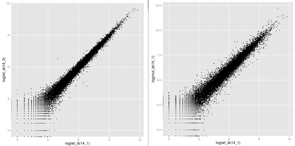
The graphs compare two wild type samples on the left and one wild type sample with one mutant on the right. Each point represents a gene and the axes are the associated expression levels. Genes with identical expression levels would appear on the diagonal. Genes up-regulated in the second sample would appear above the diagonal and down-regulated below.
Notice that the comparison between replicates of the same strain, are more similar (more tightly packed around the diagonal) than between strains - this is what you would expect. If you don’t see that most genes are not expressed at similar levels between conditions then most statistical approaches to determine differential expression will not be admissible. This is because the fundamental assumptions of these approaches assume that most genes are not differentially expressed. It may also mean you have a poorly designed experiment or noisy dataset. There are methods to deal with this which we will not cover here, but in brief, they rely upon having artificial control sequences present at known abundances or selecting housekeeping genes which are not expected to change abundance.
Further reading on this topic can be found from the following sources:
It is always good to find ways to visualise your data as it gives and intuitive understanding of what is going on. It is also important to spot errors early on in your analysis.