Now we have all of our genes loaded and have divided samples into wild-type and mutant we can now start to look at differences between strains. We can begin by looking at those genes with the most variable expression. We should have already loaded the ‘genefilter’ library.
We can now create a list of the top 20 variable genes by looking at the variation across each row.
topVarGenes = head(order(-rowVars(assay(dc14DESeqDataSet))),20)
Finally, we can view the most variable genes.
assay(dc14DESeqDataSet)[topVarGenes,]
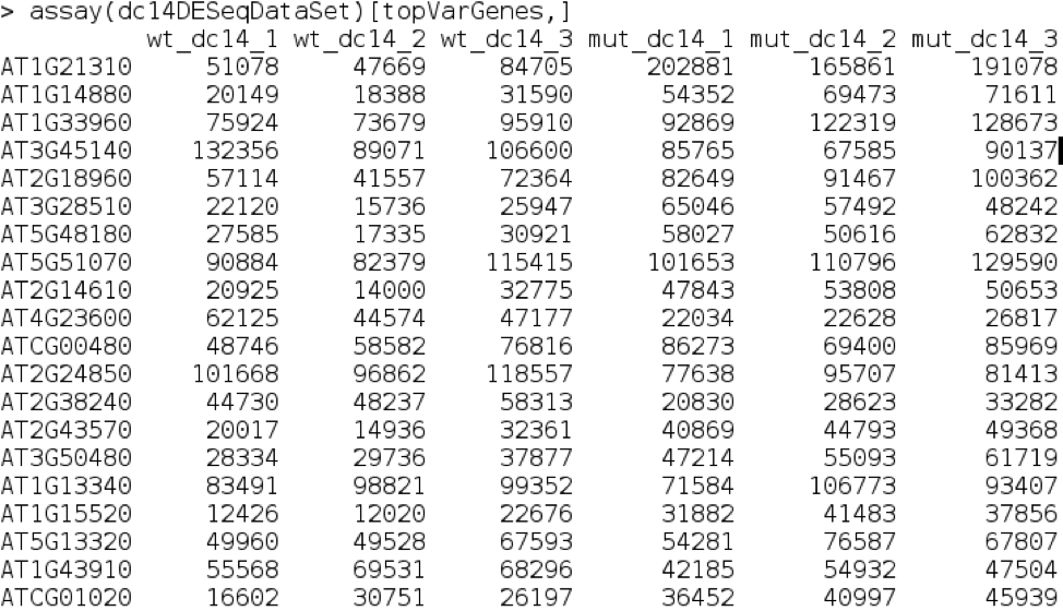
We can even look up some of these in TAIR to see if they are meaningful in the context of our experiment.
We can next look at how the 50 most variable genes cluster, but first we should do a log transformation to represent fold change rather than using the absolute count values.
dc14DESeqDataSet.rld = rlogTransformation(dc14DESeqDataSet, blind=TRUE)
Finally, we select the top 50 variably expressed genes and produce a heatmap.
topVarGenes = head(order(-rowVars(assay(dc14DESeqDataSet))),50)
mat = assay(dc14DESeqDataSet.rld)[topVarGenes,]
mat = mat - rowMeans(mat)
pheatmap(mat)
This produces the following image:
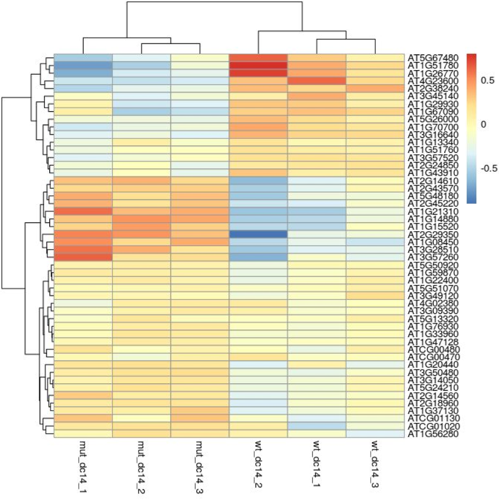
Its seems that in the top 50 most variable genes there are two major groups; (i) that shows lower gene expression in the mutant and (ii) that shows higher expression in the mutant.