Welcome to Introduction to Genomics Course

Introduction

Welcome to the Genomics workshop. Generating reams of data in Biology is easy these days. In little more than a fortnight we can generate more data than the entire human genome project generated in over a decade of work. Making biological sense out of that data, understanding its limitations and how the analysis algorithms work is now the major challenge for researchers. The aim of this workshop is to take you through a few example projects and tasks. On the way you will learn how to evaluate the quality of data as provided by a sequencing facility, how to align the data against a known and annotated reference genome and how to perform a de-novo assembly. In addition you will also learn how to compare results between different samples.

This workshop is broken into 6 parts. You should feel free to take as long as you like on each part. It is much more important that you have a thorough understanding of each part, rather than try to race through the entire workshop.

The five parts are:

• Introduction
• Remapping a strain of E.coli to a reference sequence
• Assembly of unmapped reads
• Complete de-novo assembly of all reads
• Repeating on strains of V.parahaemolyticus and comparing them
• Lon Read de-novo assembly.

For this workshop we will assume little background knowledge, except a basic familiarity with the Linux operating system and the Openstack cloud. We will cover the basics of how genomic DNA libraries are generated and sequenced, and the principles behind short read paired-end sequencing. We will look at why data can vary in quality, why adaptor sequences need to be filtered out and how to quality control data.

In the second part we will take the plunge and align the filtered reads to a reference genome, call variants and compare them against the published genome to identify missing, truncated or altered genes. This will involve the use of a publicly available set of bacterial E.coli Illumina reads and reference genome. In parts 3 and 4 we will look at how one can identify novel sequences which are not present in the reference genome. In part 5, you will be asked to repeat the steps 2, 3 and 4 on other data sets and to compare the results. In part 6 we will look at an assembly process using only long reads.

A word on notation. If you see something like this:
cd ~/genomics_tutorial/reference/sequence
It means, type the highlighted text into your terminal.

Part 1. Short Read Genomics: Introduction

Principles of Illumina-based sequencing:

There are several second generation sequencers currently on the market. These include the Ion Torrent, and many Illumina system. Other (now obsolescent) platforms included Life Tech SoLID and Roche 454. All of these systems rely on making hundreds of thousands of clonal copies of a fragment of DNA and sequencing the ensemble of fragments using DNA polymerase or in the case of the SOLiD via ligation. This is simply because the detectors (basically souped-up digital cameras), cannot detect fluorescence changes from a single molecule.

The ‘third-generation’ Pacific Biosciences SMRT (Single Molecule Real Time) Sequel sequencers are able to detect fluorescence from a single molecule of DNA. However, the machines are very large and produce less than a tenth of the data of an Illumina MiSeq run and for long reads > 0kb error rates are generally around 10-12%.

The Oxford Nanopore MinION is another ‘third-generation’ single-molecule system which measures changes in electrical current through a Nanopore as a single molecule is ratcheted through it. Although error rates are higher (5-10%) and per-base costs are higher the technology has improved rapidly and will probably replace second generation systems over the next few years. Currently however, the second generation sequencers are dominating the sequencing world.

We will mainly look at the Illumina sequencing pipeline here, but the basic principles apply to other second-generation sequencers. If you would like further details on other platforms then I recommend reading:

Mardis ER. Next-generation DNA sequencing methods. Annual Reviews Genomics Hum Genet 2008; 9 :387-402.

Goodwin S. Coming of age: ten years of next-generation sequencing technologies. Nat Rev Genet. 2016; 17:333-51.

A typical sequencing run would begin with the user supplying 1ng - 1ug of genomic DNA to a facility along with quality control information in the form of an automated electrophoresis output (e.g. Agilent Bioanalyser/Tapestation trace) or gel image and quantification information.

DNA Library preparation

For most sequencing applications, paired-end libraries are generated. Genomic DNA is sheared into 300-800 bp fragments (usually via sonication) and size-selected accordingly. Ends are repaired and an overhanging adenine base is added, after which oligonucleotide adaptors are ligated. In many cases the adaptors contain unique DNA sequences of 6-12bp which can be used to identify the sample if they are ‘multiplexed’ together for sequencing. This type of sequencing is used extensively when sequencing small genomes such as those of bacteria because it lowers the overall per-genome cost.

A) Steps a through e explain the main steps in Illumina sample preparation. B) Overview of the automated the size selection protocol.

*Borgstrom E, Lundin S, Lundeberg J, 2011 Large Scale Library Generation for High Throughput Sequencing. PLoS ONE 6:e19119. doi:10.1371/journal.pone.0019119 *

Sequencing

adapted from: (Next-Generation DNA Sequencing Methods Mardis, E.R. Annu. Rev. Genomics Hum. Genet. 2008. 9:387-402)

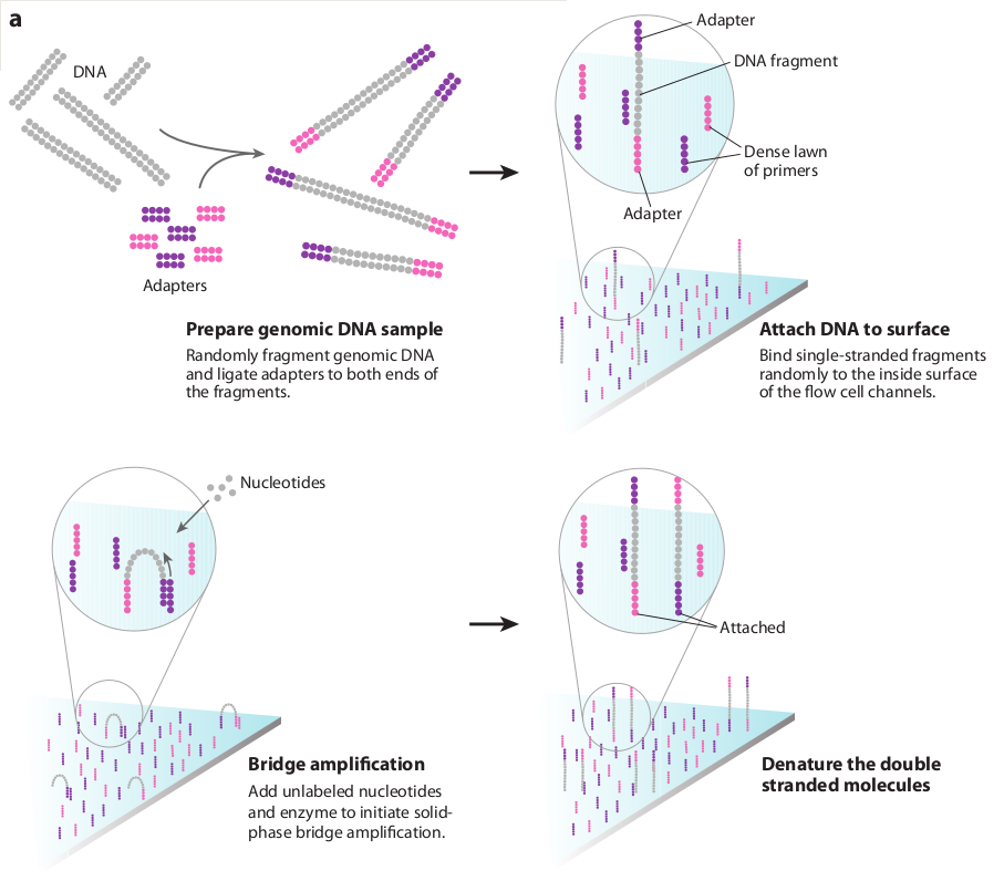
Once sufficient libraries have been prepared, the task is to amplify single strands of DNA to form monoclonal clusters. The single molecule amplification step for the Illumina HiSeq 2500 starts with an Illumina-specific adapter library and takes place on the oligo-derivatized surface of a flow cell, and is performed by an automated device called a cBot Cluster Station. The flow cell is either a 2 or 8 channel sealed glass microfabricated device that allows bridge amplification of fragments on its surface, and uses DNA polymerase to produce multiple DNA copies, or clusters, that each represent the single molecule that initiated the cluster amplification.

Separate or multiple libraries can be added to each of the eight channels, or the same library can be used in all eight, or combinations thereof. Each cluster contains approximately one million copies of the original fragment, which is sufficient for reporting incorporated bases at the required signal intensity for detection during sequencing.

The Illumina system utilizes a sequencing- by-synthesis approach in which all four nucleotides are added simultaneously to the flow cell channels, along with DNA polymerase, for incorporation into the oligo-primed cluster fragments (see figure below for details). Specifically, the nucleotides carry a base-unique fluorescent label and the 3 -OH group is chemically blocked such that each incorporation is a unique event.

An imaging step follows each base incorporation step, during which each flow cell lane is imaged in three 100-tile segments by the instrument optics at a cluster density of 600,000-800,000 per mm2. After each imaging step, the 3’ blocking group is chemically removed to prepare each strand for the next incorporation by DNA polymerase. This series of steps continues for a specific number of cycles, as determined by user-defined instrument settings, which permits discrete read lengths of 50-300 bases. A base-calling algorithm assigns sequences and associated quality values to each read and a quality checking pipeline evaluates the Illumina data from each run.
The figure below summarises the process:

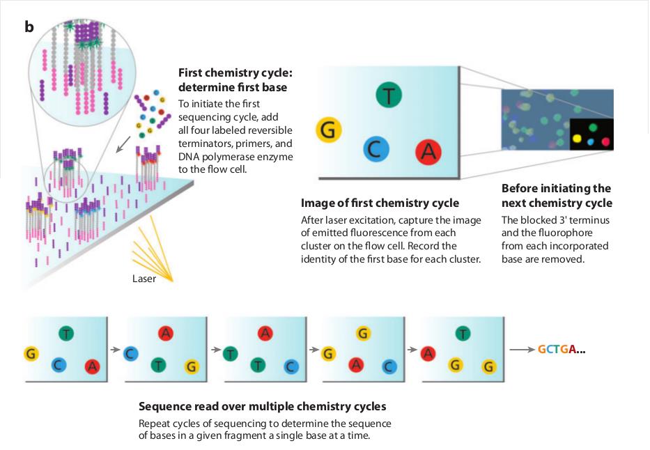
The Illumina sequencing-by-synthesis approach: Cluster strands created by bridge amplification are primed and all four fluorescently labelled, 3-OH blocked nucleotides are added to the flow cell with DNA polymerase. The cluster strands are extended by one nucleotide. Following the incorporation step, the unused nucleotides and DNA polymerase molecules are washed away, a scan buffer is added to the flow cell, and the optics system scans each lane of the flow cell by imaging units called tiles. Once imaging is completed, chemicals that effect cleavage of the fluorescent labels and the 3 -OH blocking groups are added to the flow cell, which prepares the cluster strands for another round of fluorescent nucleotide incorporation.

Base-calling involves evaluating the raw intensity values for each fluorophore and comparing them to determine which base is actually present at a given position during a cycle. To call bases on the Illumina HiSeq or SOLiD platform, the positions of clusters need to be identified during the first few cycles. This is because they are formed in random positions on the flowcell as the annealing process is stochastic. This is in contrast to the 454 system and later Illumina models where the position of each cluster is defined by a manufactured pattern in which the reaction takes place.

If there are too many clusters, the edges of the clusters will begin to merge and the image analysis algorithms will not be able to distinguish one cluster from another (remember, the software is dealing with upwards of half a million clusters per square millimeter - that’s a lot of dots!).

The above figure illustrates the principles of base-calling from cycles 1 to 9. If we focus on the highlighted cluster, one can observe that the colour (wavelength) of light observed at each cycle changes along with the brightness (intensity). This is due to the incorporation of complementary ddNTPs containing fluorophores. So at cycle 1 we have a T base, at 2 a G base and so on. If the colour or intensity is ambiguous the sequencer will mark it as an N. Other clusters are also visible in the images; these will represent different monoclonal clusters with different sequences.

The base calling algorithms turn the raw intensity values into T,G,C,A or N base calls. There are a variety of methods to do this and the one mentioned here is by no means the only one available, but it is often used as the default method on the Illumina systems, and will only call a base if the intensity divided by the sum of the highest and second highest intensity is less than a given threshold (usually 0.6). Otherwise the base is marked with an N. In addition the standard Illumina pipeline will reject an entire read if two or more of these failures occur in the first 4 bases of a read (it uses these cycles to determine the boundary of a cluster).

These processes are carried out at the sequencing facility and you will not need to perform any of these tasks under normal circumstances. They are explained here as useful background information.

Paired-end sequencing is a remarkably simple and powerful modification to the standard sequencing protocol. It is nearly always worth obtaining paired-end reads if performing genomic sequencing. Typically sequencers of any type are only able to sequence a portion of DNA (typically 125bp in the case of Illumina) before the fidelity of the enzyme and de-phasing of clusters (see later) increase the error rate beyond tolerable levels. As a result, on the Illumina system, a fragment which is 500bp long will only have the first 125bp sequenced.

If the size selection is tight enough and you know that nearly all the fragments are close to 500bp long, you can repeat the sequencing reaction from the other end of the fragment. This will yield two reads for each DNA fragment separated by a known distance. In the figure below the dashed regions represent the complete DNA fragment and the solid lines the regions we are able to sequence:

The added information gained by knowing the distance between the two reads can be invaluable for spanning repetitive regions. In the figure below, the light coloured regions indicate repetitive sections of DNA. If a read contains only repetitive DNA, an alignment algorithm will be able to map the read to many locations in a reference genome. However, with paired-end reads, there is a greater chance that

at least one of the two reads will map to a unique region of DNA. In this way one of the reads can be used to anchor the other read in the pair and help resolve the repetitive region. Paired-end reads are often used when performing de-novo genome sequencing (i.e. when a reference is not available to align against) because they enable contiguous regions of DNA to be ordered, or when characterizing variants such as large insertions or deletions.

Other forms of paired-end sequencing with much larger distances (e.g. 10kb) are possible with so called ‘mate-pair’ libraries. These are usually used in specific projects to help order contigs in de-novo sequencing projects. We will not cover them here, but the principles behind them are similar.

Inherent sources of error

No measurement is without a certain degree of error. This is true in sequencing. As such there is a finite probability that a base will not be called correctly. There are several possible sources:

Frequency cross-talk and normalisation errors:

When reading an A base, a small amount of C will also be measured due to frequency overlap and vice-versa. Similarly with G and T bases. Additionally, from the figure below, it should be clear that the extent to which the dyes fluoresce differs. As such it is necessary to normalize the intensities. This normalisation process can also introduce errors.

Frequency response curve for A and C dyes

(Intensity y-axis and frequency on the x-axis) **

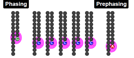
Phasing/Pre-phasing:

his occurs when a strand of DNA lags or leads the other DNA strands within a cluster. This introduces additional background noise into the signal and reduces the intensity of the true base. In the example below we have a cluster with 7 strands of DNA (very small, but this is just an example). Five strands are on a C-base, whilst 1 is lagging behind (called phasing) on a G base and the remaining strand is running ahead of the pack (confusingly called pre-phasing) on an A base. As such the C signal will be reduced and A and G boosted for the rest of the sequencing run. Too much phasing or pre-phasing (i.e. > 15-20%) usually causes problems for the base calling algorithm and result in clusters being filtered out.

Other issues:

Biases introduced by sample preparation - your sequencing is only as good as your experimental design and DNA extraction. Remember that your sample will be put through several cycles of PCR before sequencing which is also introduces a potential source of bias.

High AT or GC content sequences - reduces the complexity of the sequence and can result in higher error rates.

Homopolymeric sequences - long stretches of a single base can make it difficult to determine phasing and pre-phasing rates. This can introduce errors in determining the precise length of a hompolymeric stretch of sequence. This much more of a problem on the 454 and Ion Torrent than Illumina platforms but still worth bearing in mind. Especially if you encounter indels which have been called in homopolymeric tracts.

Certain motifs can cause loops and other steric clashes See Nakamura et al, Sequence-specific error profile of Illumina sequencers Nuc. Acid Res. first published online May 16, 2011 doi:10.1093/nar/gkr344

Understanding Quality scores

To account for the possible errors and provide an estimate of confidence in a given base-call, the Illumina sequencing pipeline assigns a quality score to each base called. Most quality scores are calculated using the Phred scale. Each base call has an associated base call quality which estimates the chance that the base call is incorrect.

Q10 = 1 in 10 chance of incorrect base call
Q20 = 1 in 100 chance of incorrect base call
Q30 = 1 in 1000 chance of incorrect base call
Q40 = 1 in 10,000 chance of incorrect base call

For most 454, SOLiD and Illumina runs you should see quality scores between Q20 and Q40. Note that these as only estimates of base-quality based on calibration runs performed by the manufacturer against a sample of known sequence with (typically) a GC content of 50%. Extreme GC bias and/or particular motifs or homopolymers can cause the quality scores to become unreliable.

Accurate base qualities are an essential part in ensuring variant calls are correct. As a rough and ready rule we generally assume that with Illumina data anything less than Q20 is not useful data and should be excluded from the analysis.

Reads containing adaptors

Some reads will contain adaptor sequences after sequencing, usually at the end of the read. This is usually because of short sample DNA fragments, which result in the polymerase reading into the adaptor region. Occasionally this can also happen because of mis-priming. It is important to remove or trim sequences containing these reads as the adaptor sequences can prevent reads mapping to a reference sequence and will adversely affect de-novo assembly

Part 2. Short Read Genomics: Remapping

In this section of the workshop we will be analysing a strain of E.coli which was sequenced at Exeter. It is closely related to the K-12 substrain MG1655 (http://www.ncbi.nlm.nih.gov/nuccore/U00096). We want to obtain a list of single nucleotide polymorphisms (SNPs), insertions/deletions (Indels) and any genes which have been deleted.

Quality control

In this section of the workshop we will be learning about evaluating the quality of an Illumina MiSeq sequencing run. Sequencing data is usually delivered in FASTQ format and the process described here can be used with any FASTQ formatted file from any platform (e.g 454, Illumina, Ion Torrent, PacBio etc).

2nd (and 3rd) generation sequencers produce vast quantities of data. A single Illumina MiSeq lane will produce over 10-Gbases of data. However, the error rates of these platforms are 10-100x higher than Sanger sequencing. They also have very different error profiles. Unlike Sanger sequencing, where the most reliable sequences tend to be in the middle, NGS platforms tend to be most reliable near the beginning of each read.

Quality control usually involves:

• Calculating the number of reads before quality control
• Calculating GC content, identifying over-represented sequences
• Remove or trim reads containing adaptor sequences
• Remove or trim reads containing low quality bases
• Calculating the number of reads after quality control
• Rechecking GC content, identifying over-represented sequences

Quality control is necessary because:

• CPU time required for alignment and assembly is reduced
• Data storage requirements are reduced
• Reduce potential for bias in variant calling and/or de-novo assembly

Quality scores

Most quality scores are calculated using the Phred scale (Ewing B, Green P: Basecalling of automated sequencer traces using phred. II. Error probabilities. Genome Research 8:186-194 (1998)).

Each base call has an associated base call quality which estimates chance that the base call is incorrect.

Q10 = 1 in 10 chance of incorrect base call
Q20 = 1 in 100 chance of incorrect base call
Q30 = 1 in 1000 chance of incorrect base call
Q40 = 1 in 10,000 chance of incorrect base call

For most 454, SoLID and Illumina runs you should see quality scores between Q20 and Q40. Note that these as only estimates of base-quality based on calibration runs performed by the manufacturer against a sample of known sequence with (typically) a GC content of 50%. Extreme GC biases and/or particular motifs or homopolymers can cause the quality scores to become unreliable. Accurate base qualities are an essential part in ensuring variant calls are correct. As a rough and ready rule we generally assume that with Illumina data anything less than Q20 is not useful data and should be excluded.

Once you understand the FASTQ format try to work out what is happing to the quality scores here and why - A FASTQ entry consists of 4 lines:

line 1 - A header line beginning with ‘@’ containing information about the name of the sequencer, and the position at which the originating cluster was located and whether it passed purity filters.
line 2 - The DNA sequence of the read
line 3 - A header line or line beginning with just ‘+’
line 4 - Quality scores for each base encoded in ASCII format

To reduce storage requirements, the FASTQ quality scores are stored as single characters and converted to numbers by obtaining the ASCII quality score and subtracting either 33 (or 64 for much older datasets). For example, the above FASTQ file is Sanger formatted and the character ! has an ASCII value of 33. Therefore the corresponding base would have a Phred quality score of 33-33=Q0 (i.e. totally unreliable). On the other hand a base with a quality score denoted by @ has an ASCII value of 64 and would have a Phred quality score of 64-33=Q31 (i.e. less than 1/1000 chance of being incorrect).

Happily the community has pretty much standardized on base 33 encoding, but do be aware that older datasets may use a different offset for encoding.

The first task when one receives sequencing data is to evaluate its quality and determine whether all the cash you have handed over was well-spent! To do this we will use the FastQC toolkit (http://www.bioinformatics.bbsrc.ac.uk/projects/fastqc/). FastQC offers a graphical visualisation of QC metrics, but does not have the ability to filter data.

Task 1 From your home directory change into the workshop_materials/genomics_tutorial/data/sequencing/ecoli_exeter/ directory and list the directory contents. E.g.:

cd ~/workshop_materials/genomics_tutorial/data/sequencing/ecoli_exeter
ls -l

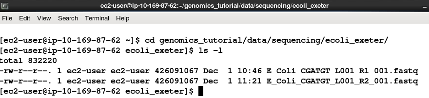
Note that this is a paired-end run. As such there are two files:

• one for read 1 (E_Coli_CGATGT_L001_R1_001.fastq)
• and the other for the reverse read 2 (E_Coli_CGATGT_L001_R2_001.fastq)

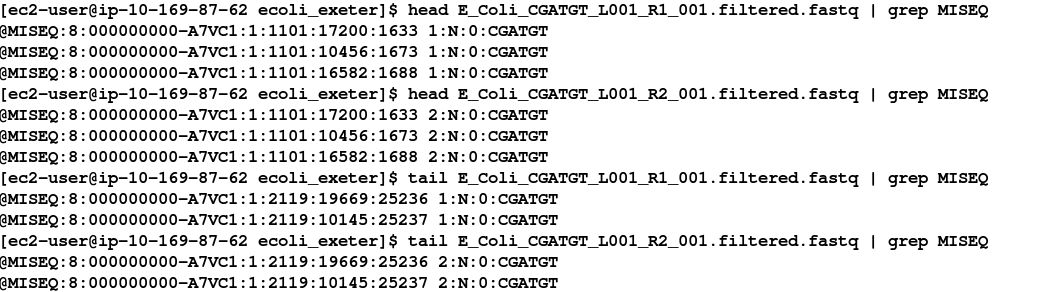
Reads from the same pair can be identified because they have the same header. Programs which use FASTQ files generally require that the read 1 and read 2 files have the reads in the same order. To view the first few headers we can use the head and grep commands:

head E_Coli_CGATGT_L001_R1_001.fastq | grep MISEQ
head E_Coli_CGATGT_L001_R2_001.fastq | grep MISEQ  

The only difference in the headers for the two reads is the read number. Of course this is no guarantee that all the headers in the file are consistent. To get some more confidence repeat the above commands using ‘tail’ instead of ‘head’ to compare reads at the end of the files.

You can also check that there is an identical number of reads in each file using cat, grep and wc -l:

cat E_Coli_CGATGT_L001_R1_001.fastq | grep MISEQ | wc -l
cat E_Coli_CGATGT_L001_R2_001.fastq | grep MISEQ | wc -l

Task 2

Now, let’s start the fastqc program.
fastqc

Load the E_Coli_CGATGT_L001_R1_001.fastq file from the workshop_materials/genomics_tutorial/data/sequencing/ecoli_exeter directory.

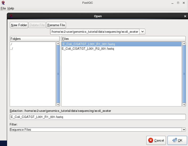
After a few minutes the program should finish analysing the FASTQ file.

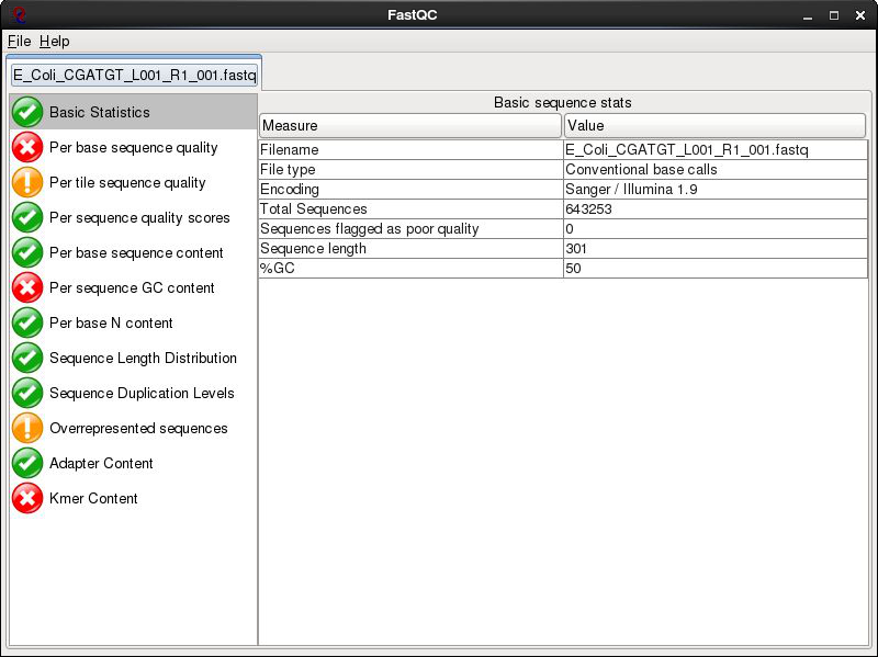
The fastqc program performs a number of tests which determines whether a green tick (pass), exclamation mark (warning) or red cross (fail) is displayed. However it is important to realise that fastqc has no knowledge of what your library is or should look like.

All of its tests are based on a completely random library with 50% GC content. Therefore if you have a sample which does not match these assumptions, it may ‘fail’ the library. For example, if you have a high AT or high GC organism it may fail the per sequence GC content. If you have any barcodes or low complexity libraries (e.g. small RNA libraries) they may also fail some of the sequence complexity tests.

The bottom line is that you need to be aware of what your library is and whether what fastqc is reporting makes sense for that type of library. In this case we have a number of errors and warnings which at first sight suggest there has been a problem - but don’t worry too much yet. Let’s go through them in turn.

Per Base Sequence Quality is one of the most important metrics. This view shows an overview of the range of quality values across all bases at each position in the FASTQ file. Generally anything with a median quality score greater than Q20 is regarded as acceptable; anything above Q30 is regarded as ‘good’. For more details, see the help documentation in fastqc.

In this case this check is red - and it is true that the quality drops off at the end of the reads. It is normal for read quality to get worse towards the end of the read. You can see that at 250 bases the quality is still very good, we will later trim off the low quality bases so reserve judgment for now.

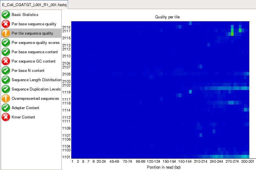Per tile sequence quality is a purely technical view on the sequencing run, it is more important for the team running the sequencer. The sequencing flowcell is divided up into areas called cells. You can see that the read quality drops off in some cells faster than others. This maybe because of the way the sample flowed over the flowcell or a mark or smear on the lens of the optics.

Per base sequence content For a completely randomly generated library with a GC content of 50% one expects that at any given position within a read there will be a 25% chance of finding an A, C, T or G base. Here we can see that our library satisfies these criteria, although there appears to be some minor bias at the beginning of the read. This may be due to PCR duplicates during amplification or during library preparation. It is unlikely that one will ever see a perfectly uniform distribution. See http://sequencing.exeter.ac.uk/guide-to-your-data/quality-control for examples of good vs bad runs as well as the fastqc help for more details.

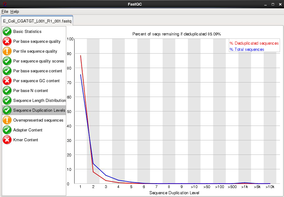
Sequence Duplication Levels In a library that covers a whole genome uniformly most sequences will occur only once in the final set. A low level of duplication may indicate a very high level of coverage of the target sequence, but a high level of duplication is more likely to indicate some kind of enrichment bias (e.g. PCR over- amplification). This module counts the degree of duplication for every sequence in the set and creates a plot showing the relative number of sequences with different degrees of duplication.

Overrepresented Sequences This check for sequences that occur more frequently than expected in your data. It also checks any sequences it finds against a small database of known sequences. In this case it has found that a small number of reads 4000 out of 600000 appear to contain a sequence used in the preparation for the library. A typical cause is that the original DNA was shorter than the length of the read - so the sequencing overruns the actual DNA and runs in to the adaptors used to bind it to the flowcell. At this level there is nothing to worry about - they will be trimmed in later stages.

There are other reports available - Have a look at them and at what the author of FastQC has to say.

https://www.bioinformatics.babraham.ac.uk/projects/fastqc/Help/3%20Analysis%20Modules/

Remember the error and warning flags are his (albeit experienced) judgement of what typical data should look like. It is up to you to use some initiative and understand whether what you are seeing is typical for your dataset and how that might affect any analysis you are performing.

Do the same for read 2 as we have for read 1. Open fastqc and analyse the read 2 file. Look at the various plots and metrics which are generated. How similar are they? Note that the number of reads reported in both files is identical. This is because if one read fails to pass the Illumina chastity filter, its partner is automatically excluded too. Overall, both read 1 and read 2 can be regarded as ‘good’ data-sets.

Quality filtering of Illumina data

In this section we will be filtering the data to ensure any low quality reads are removed and that any sequences containing adaptor sequences are either trimmed or removed altogether. To do this we will use the fastq-mcf program from the ea-utils package (available at https://expressionanalysis.github.io/ea-utils/). This package is remarkably fast and ensures that after filtering both read 1 and read 2 files are in the correct order.

Note: Typically when submitting raw Illumina data to NCBI or EBI you would submit unfiltered data, so don’t delete your original fastq files!

A note on checking for contaminants:

A number of tools are available now which also enable to you to quickly search reads and assign them to particular species or taxonomic groups. These can serve as a quick check to make sure your samples or libraries are not contaminated with DNA from other sources. If you are performing a de-novo assembly for example and have unwittingly have DNA sequence present from multiple organisms, you will risk poor results and chimeric contigs. Some ‘contaminants’ can turn out to be inevitable by-products of sampling and DNA extraction. This is often the case with algae or other symbionts. In addition some groups have made some amazing discoveries such as the discovery of a third symbiont (which turned out to be a yeast) in lichen. http://science.sciencemag.org/content/353/6298/488.full

Some tools you can use to check the taxonomic classification of reads include We won’t do this now but will do an example in the final section of the workshop on long reads.

• Kraken
• Centrifuge
• Blobology
• Blast (in conjunction with sub-sampling your reads) and Krona to plot results

Task 3

Make sure you are in the correct directory:

cd ~/workshop_materials/genomics_tutorial/data/sequencing/ecoli_exeter/

We will execute the fastq-mcf program which performs both adaptor sequence trimming and low quality bases. To remove adaptor sequences, we need to supply the adaptor sequences to the program. A list of the most common adaptors used is given in the file:

~/workshop_materials/genomics_tutorial/data/reference/adaptors/adaptors.fasta

View it by typing:

less ~/workshop_materials/genomics_tutorial/data/reference/adaptors/adaptors.fasta  

Now to run the fastq-mcf program, type the following (all on one line):

fastq-mcf ../../reference/adaptors/adaptors.fasta E_Coli_CGATGT_L001_R1_001.fastq E_Coli_CGATGT_L001_R2_001.fastq -o E_Coli_CGATGT_L001_R1_001.filtered.fastq -o E_Coli_CGATGT_L001_R2_001.filtered.fastq -C 1000000 -q 20 -p 10 -u -x 0.01

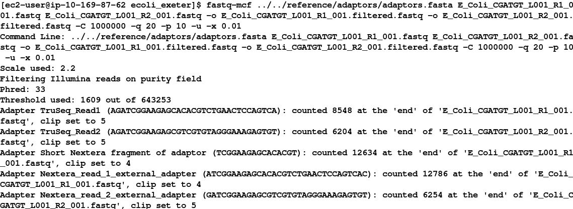
While this is running enter the command fastq-mcf in another terminal and try to understand what the options we are using do. We have found that these parameters generally work well for Illumina data. If you would like to learn more about these options, you can look at the manual here: https://github.com/ExpressionAnalysis/ea-utils/blob/wiki/FastqMcf.md.

In short we are using 1 million reads to form a model of the sequence quality and then applying the filters which remove bases with q-score less than 20, trims adaptors allowing up to 10% mismatch in the adaptor sequence, allowing only pass-filter reads (virtually all sequencing data is pass-filter these days, so this is just included to be safe) and trims back reads which contain more than 1% Ns until they contain 1% or less Ns.

After a few minutes the filtering should be complete and you should see something similar to:

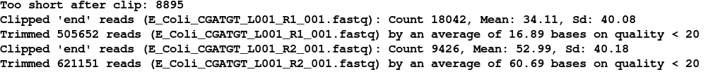
You can see that the trimming has been harsher on the R2 reads than on the R1 - this is generally to be expected in Illumina paired end runs. If we look at the sizes of the files produced:

ls -l

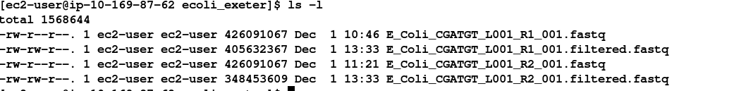
You can see that the original files are exactly the same size, but the R2 filtered file is smaller than R1. Now count the lines in all the files:

wc -l *.filtered.fastq

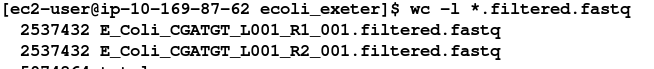
Although the reads have been trimmed differently - the number of reads in the R1 and R2 files are identical. This is required for all the tools we will use to analyse paired end data.

Task 4

Check the quality scores and sequence distribution in the fastqc program for the two filtered fastq files. You should notice very little change (since comparatively few reads were filtered).

However, you should notice a significant improvement in quality and the absence of adaptor sequences.

Task 5

We can perform a quick check (although this by no means guarantees) that the sequences in read 1 and read 2 are in the same order by checking the ends of the two files and making sure that the headers are the same.

head E_Coli_CGATGT_L001_R1_001.filtered.fastq | grep MISEQ
head E_Coli_CGATGT_L001_R2_001.filtered.fastq | grep MISEQ
tail E_Coli_CGATGT_L001_R1_001.filtered.fastq | grep MISEQ
tail E_Coli_CGATGT_L001_R2_001.filtered.fastq | grep MISEQ

Check the number of reads in each filtered file. They should be the same. To do this use the grep command to search for the number of times the header appears. E.g:

grep -c MISEQ E_Coli_CGATGT_L001_R1_001.filtered.fastq

Do the same for the E_Coli_CGATGT_L001_R2_001.filtered.fastq file.

Task 6

Aligning Illumina data to a reference sequence

Now that we have checked the quality of our raw data, we can begin to align the reads against a reference sequence. In this way we can compare how the reference sequence and the strain we have sequenced compare.

To do this we will be using a program called BWA (Burrows Wheeler Aligner Li H. and Durbin R. (2009) Fast and accurate short read alignment with Burrows-Wheeler Transform. Bioinformatics, 25:1754-60. ). This uses an algorithm called (unsurprisingly) Burrows Wheeler to rapidly map reads to the reference genome. BWA also allows for a certain number of mismatches to account for variants which may be present in strain 1 vs the reference genome. Unlike other alignment packages such as Bowtie (version 1) BWA allows for insertions or deletions as well.

By mapping reads against a reference, what we mean is that we want to go from a FASTQ file listing lots of reads, to another type of file (which we’ll describe later) which lists the reads AND where/if it maps against the reference genome.

The figure below illustrates what we are trying to achieve here. Along the top in grey is the reference sequence. The coloured sequences below indicate individual sequences and how they map to the reference. If there is a real variant in a bacterial genome we would expect that (nearly) all the reads would contain the variant at the relevant position rather than the same base as the reference genome. Remember that error rates for any single read on second generation platforms tend to be around 0.5-1%. Therefore a 300bp read is on average likely to contain at 2-3 errors.

Let’s look at 2 potential sources of artefacts.

Sequencing error:

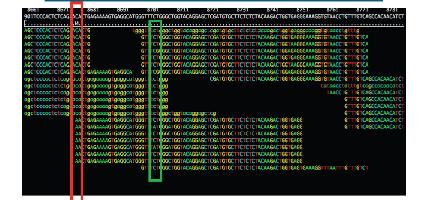
The region highlighted in green above shows that most reads agree with the reference sequence (i.e. C-base). However, 2 reads near the bottom show an A-base. In this situation we can safely assume that the A-bases are due to a sequencing error rather than a genuine variant since the ‘variant’ has only one read supporting it. If this occurred at a higher frequency however, we would struggle to determine whether it was a genuine variant or an error.

PCR duplication:

The highlighted region red above shows where there appears to be a variant. A C-base is present in the reference and half the reads, whilst an A-base is present in a set of reads which all start at the same position.

Is this a genuine difference or a sequencing or sample prep error? What do you think? If this was a real sample, would you expect all the reads containing an A to start at the same location?

The answer is probably not. This ‘SNP’ is in fact probably an artefact of PCR duplication. I.e. the same fragment of DNA has been replicated many times more than the average and happens to contain an error at the first position. We can filter out such reads during after alignment to the reference (see later).

Note that the entire region above seems to contain lots of PCR duplicates with reads starting at the same location. In the case of the region highlighted in red, this will likely cause a false SNP call. The area in green also contains PCR duplicates the As at these positions are probably either sequencing errors or errors introduced during PCR.

It’s always important to think critically about any finding - don’t assume that whatever bioinformatic tools you are using are perfect. Or that you have used them perfectly.

Indexing a reference genome:

Before we can start aligning reads to a reference genome, the genome sequence needs to be indexed. This means sorting the genome into easily searched chunks.

Task 7

Generating an index file from the reference sequence

Change directory to the reference directory, and list the files:

cd ~/workshop_materials/genomics_tutorial/data/reference/U00096/
ls -l

In this directory we have 2 files. U00096.fna is a FASTA file which contains the reference genome sequence. The U00096.gff file contains the annotation for this genome. We will use this later.

First, let’s looks at the bwa command itself. Type:

bwa

This should yield something like:

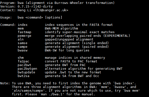
BWA is actually a suite of programs which all perform different functions. We are only going to use two during this workshop, bwa index, bwa mem

If we type:

bwa index

We can see more options for the bwa index command.

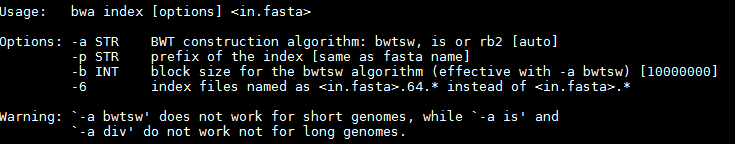
By default bwa index will use the IS algorithm to produce the index. This works well for most genomes, but for very large ones (e.g. vertebrate) you may need to use bwtsw. For bacterial genomes the default algorithm will work fine.

Now we will create a reference index for the genome using BWA:

bwa index U00096.fna

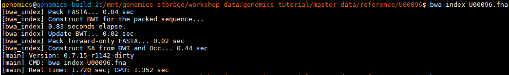
If you now list the directory contents using the ‘ls’ command, you will notice that the BWA index program has created a set of new files. These are the index files BWA needs.

Task 8: Aligning reads to the indexed reference sequence.

Now we can begin to align read 1 and read 2 to the reference genome. First of all change back into the ~/workshop_materials/genomics_tutorial/data/sequencing/ecoli_exeter/ directory and create a subdirectory to contain our remapping results.

cd ~/workshop_materials/genomics_tutorial/data/sequencing/ecoli_exeter/
mkdir remapping_to_reference
cd remapping_to_reference

Let’s explore the alignment options BWA MEM has to offer. Type:

bwa mem

The basis format of the command is:

Usage: bwa mem [options] [in2.fq]

We can see that we need to provide BWA with a FASTQ files containing the raw reads (denoted by and ) to align to a reference file (unhelpfully this is listed as ).

There are also a number of options. The most important are

• the maximum number of differences in the seed (-k i.e. the first 32 bp of the sequence vs the reference),
• the number of processors the program should use (-t - our machine has 8 processors).

Our reference sequence is in ~/workshop_materials/genomics_tutorial/data/reference/U00096/U00096.fna

Our filtered reads in:
~/workshop_materials/genomics_tutorial/data/sequencing/ecoli_exeter/E_Coli_CGATGT_L001_R1_001.filtered.fastq
~/workshop_materials/genomics_tutorial/data/sequencing/ecoli_exeter/E_Coli_CGATGT_L001_R2_001.filtered.fastq

So to align our paired reads using processors and output to file E_Coli_CGATGT_L001_filtered.sam:

type, all on one line:

bwa mem -t 8 ~/workshop_materials/genomics_tutorial/data/reference/U00096/U00096.fna ~/workshop_materials/genomics_tutorial/data/sequencing/ecoli_exeter/E_Coli_CGATGT_L001_R1_001.filtered.fastq ~/workshop_materials/genomics_tutorial/data/sequencing/ecoli_exeter/E_Coli_CGATGT_L001_R2_001.filtered.fastq > E_Coli_CGATGT_L001_filtered.sam

There will be quite a lot of output but the end should look like:

Once the alignment is complete, list the directory contents and check that the alignment file is present. ls -lh

Note: ls -lh outputs the size of the file in human readable format (780Mb in this case - don’t worry if yours are slightly different.

The raw alignment is stored in what is called SAM format (Simple AlignMent format). It is in plain text format and you can view it if you wish using the ‘less’ command. Do not try to open the whole file in a text editor as you will likely run out of memory!

less E_Coli_CGATGT_L001_filtered.sam

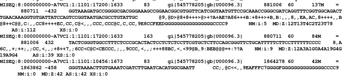
Each alignment line has 11 mandatory fields for essential alignment information such as mapping position, and a variable number of optional fields for flexible or aligner specific information. For further details as to what each field means see http://samtools.sourceforge.net/SAM1.pdf

Task 9: Convert SAM to BAM file

Before we can visualise the alignment however, we need to convert the SAM file to a BAM (Binary AlignMent format) which can be read by most software analysis packages. To do this we will use another suite of programs called samtools. Type:

samtools view

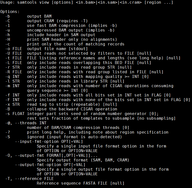
We can see that we need to provide samtools view with a reference genome in FASTA format file (-T), the -b and -S flags to say that the output should be in BAM format and the input in SAM, plus the alignment file.

Remember our reference sequence is in ~/workshop_materials/genomics_tutorial/data/reference/U00096/U00096.fna

Type (all on one line):

samtools view -bS --threads 8 -T  ~/workshop_materials/genomics_tutorial/data/reference/U00096/U00096.fna E_Coli_CGATGT_L001_filtered.sam > E_Coli_CGATGT_L001_filtered.bam

Aside: Many commands can run in multiple processes often called threads, which will reduce the runtime of many commands - for samtools it is the the --threads option. Out of interest try a few different values. You can prefix your command with time to capture the runtime easily.
samtools view -bS -T --threads xx ..etc..
try a few different values e.g. 4,8,16 - do you understand the pattern?

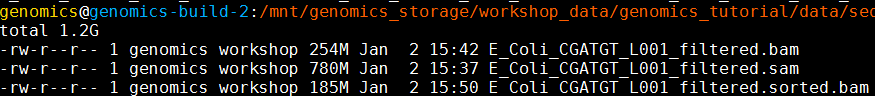
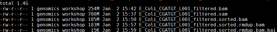
ls -lh

It’s always good to check that your files have processed correctly if something goes wrong it’s better to catch it immediately.

Note that the bam file is smaller than the sam file - this is to be expected as the binary format is more efficient.

Task 10: Sort BAM file

Once this is complete we then need to sort the BAM file so that the reads are stored in the order they appear along the chromosomes (don’t ask me why this isn’t done automatically….). We can do this using the samtools sort command.

samtools sort --threads 8 E_Coli_CGATGT_L001_filtered.bam -o E_Coli_CGATGT_L001_filtered.sorted.bam

This will take another minute or so. Don’t forget to check the resulting file.

A note on piping BWA and samtools commands: In tasks 8-10 we aligned reads to the reference genome, converted SAM to BAM and then sorted the resulting BAM file. For clarity we have shown these as individual steps. However, in real-life, it is faster and easier to do these simultaneously using Unix pipes!

E.g. (there is no need to do this)

bwa mem -t 2 ~/workshop_materials/genomics_tutorial/data/reference/U00096/U00096.fna ~/workshop_materials/genomics_tutorial/data/sequencing/ecoli_exeter/E_Coli_CGATGT_L001_R1_001.filtered.fastq ~/workshop_materials/genomics_tutorial/data/sequencing/ecoli_exeter/E_Coli_CGATGT_L001_R2_001.filtered.fastq > E_Coli_CGATGT_L001_filtered.sam | samtools sort -O bam -o E_Coli_CGATGT_L001_filtered.sorted.bam

Task 11: Remove suspected PCR duplicates

Especially when using paired-end reads, samtools can do a reasonably good job of removing potential PCR duplicates (see the first part of this workshop if you are unsure what this means).

Again, samtools has a command to do this called rmdup.

samtools rmdup E_Coli_CGATGT_L001_filtered.sorted.bam E_Coli_CGATGT_L001_filtered.sorted.rmdup.bam

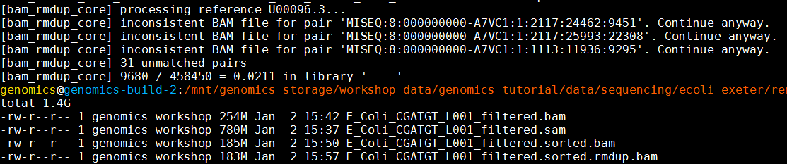
You will notice some warnings about inconsistent BAM file for pair - this is just a warning that a pair of reads does not align together on the genome within the expected tolerance - it is normal to expect some of these, and you can ignore.

Task 12: Index the BAM file

Most programs used to view BAM formatted data require an index file to locate the reads mapping to a particular location quickly. You can think of this as an index in a book, telling you where to go to find particular phrases or words. We’ll use the samtools index command to do this.

samtools index E_Coli_CGATGT_L001_filtered.sorted.rmdup.bam

We should obtain a .bai file (known as a BAM-index file).

Task 13: Obtain mapping statistics

Finally we can obtain some summary statistics.

samtools flagstat E_Coli_CGATGT_L001_filtered.sorted.rmdup.bam > mappingstats.txt

This should only take a few seconds. Once complete view the mappingstats.txt file using a text-editor (e.g. gedit or nano) or the ‘more’ command.

So here we can see we have 1250574 reads in total, none of which failed QC. 71.88% of reads mapped to the reference genome and 71.55% mapped with the expected 500-600bp distance between them. 1414 reads could not have their read-pair mapped.

0 reads have mapped to a different chromosome than their pair (0 has a mapping quality > 5 - this is a Phred scaled quality score much as we say in the FASTQ files). If there were any such reads they would likely due to repetitive sequences (e.g phage insertion sites) or an insertion of plasmid or phage DNA into the main chromosome.

Task 14: Cleanup We have a number of leftover intermediate files which we can now remove to save space.

Type (all on one line):

rm E_Coli_CGATGT_L001_filtered.sam E_Coli_CGATGT_L001_filtered.bam E_Coli_CGATGT_L001_filtered.sorted.bam

In case you get asked if you are sure to remove 3 arguments type in ‘yes’ and hit enter. You should now be left with the processed alignment file, the index file and the mapping stats.

Well done! You have now mapped, filtered and sorted your first whole genome data-set! Let’s take a look at it!

Task 15: QualiMap

Qualimap (http://qualimap.bioinfo.cipf.es/) is a program that summarises the alignment in much more detail than the mapping stats file we produced. It’s a technical tool which allows you to assess the sequencing for any problems and biases in the sequencing and the alignment rather than a tool to deduce biological features.

There are a few options to the program, We want to run bamqc. Type:
qualimap bamqc
to get some help on this command.

To get the report, first make sure you are in the directory: ~/workshop_materials/genomics_tutorial/data/sequencing/ecoli_exeter/remapping_to_reference then run the command:

qualimap bamqc -outdir bamqc -bam E_Coli_CGATGT_L001_filtered.sorted.rmdup.bam -gff ~/workshop_materials/genomics_tutorial/data/reference/U00096/U00096.gff

this creates a subfolder called bamqc

cd to this directory and run
firefox qualimapReport.html

There is a lot in the report so just a few highlights:

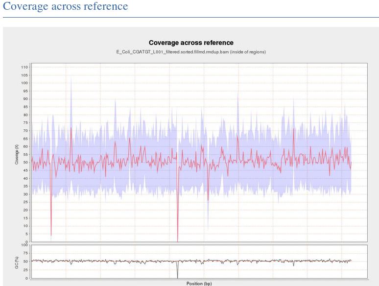
This shows the numbe of reads that ‘cover’ each section of the genome. The red line shows a rolling average around 50x - this means that on average every part of the genome was sequenced 50X. It is important to have sufficient depth of coverage in order to be confident that any features you find in your data are real and not a result of sequencing errors.

What do you think the regions of low/zero coverage correspond to?

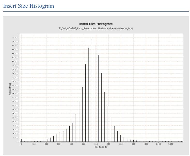
The Insert Size Histogram displays the range of sizes of the DNA fragments. It shows how well your DNA was size selected before sequencing. Note that the ‘insert’ refers to the DNA that was inserted between the sequencing adaptors, so equates to the size range of the DNA that was used. In this case we have 300 paired end reads and our insert size varies around 600 bases - so there should only be a small gap between the reads that was not sequenced.

Have a look at some of the other graphs produced.

Task 16: Load the Integrative Genomics Viewer

The Integrative Genome Viewer (IGV) is a tool developed by the Broad Institute for browsing interactively the alignment data you produced. It has a wealth of features and we can only cover some basics to get you started. Go to http://www.broadinstitute.org/igv/ to get more information.

In your terminal, type igv.sh Or you can click the icon on the desktop. IGV viewer should appear:

Notice that by default a human genome has been loaded.

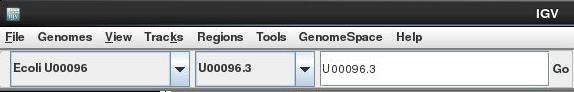
Task 17: Import the E.coli U0009 reference genome to IGV

By default IGV does not contain our reference genome. We’ll need to import it.

Click on ‘Genomes ->Create .genome file…’

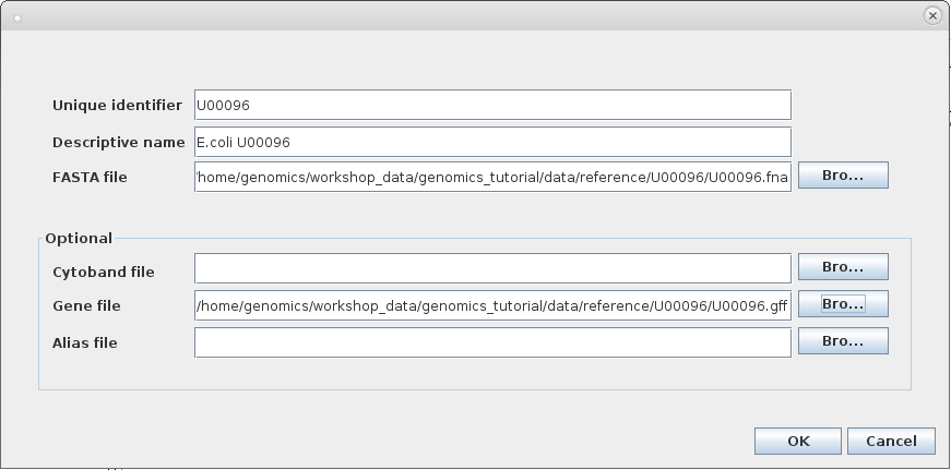
Enter the information above and click on ‘OK’ .

IGV will ask where it can save the genome file. Your home directory will be fine.

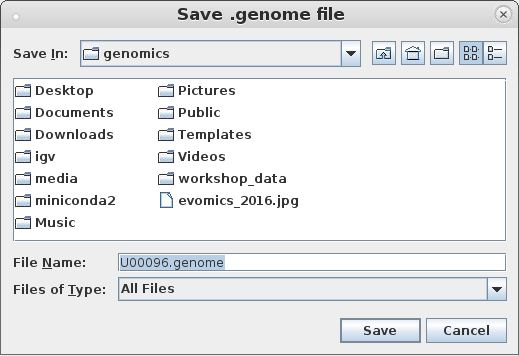
Click ‘Save’ again.

Note that the genome and the annotation have now been imported.

Task 18: Load the BAM file

Load the alignment file. Note that IGV requires the .bai index file to also be in the same directory.

Select File… and Load From File

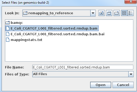
Select the bam file and click open

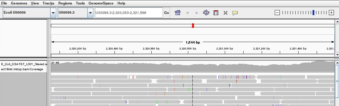
Once loaded your screen should look similar to the following. Note that you can load more BAM files if you wish to compare different samples or the results of different mapping programs.

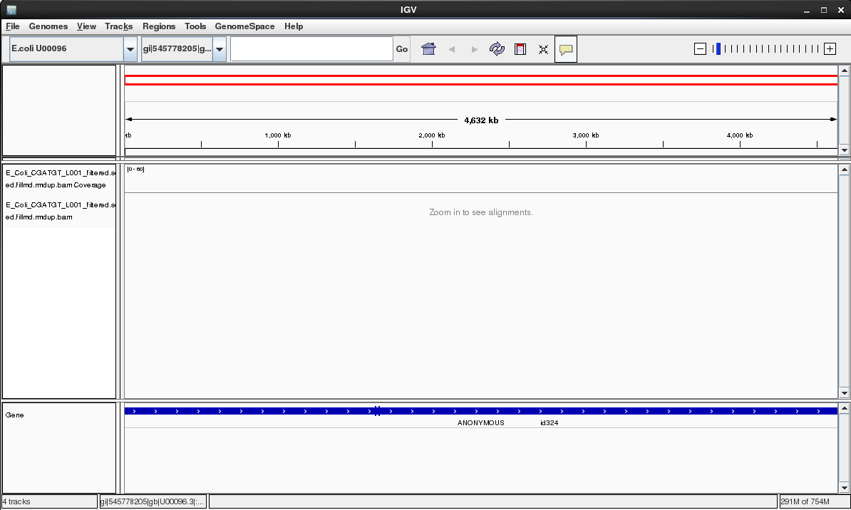
Select the chromosome U00096.3 if it is not already selected

Use the +/- keys to zoom in or use the zoom bar at the top right of the screen to zoom into about 1-2kbases as below:

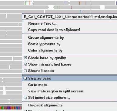
Right click on the main area and select view as pairs

The gray graph at the top of the figure indicates the coverage of the genome:

The more reads mapping to a certain location, the higher the peak on the graph. You’ll see a coloured line of blue, green or red in this coverage plot if there are any SNPs (single-nucleotide polymorphisms) present (there are none in the plot).

If there are any regions in the genome which are not covered by the reads, you will see these as gaps in the coverage graph. Sometimes these gaps are caused by repetitive regions; others are caused by genuine insertions/deletions in your new strain with respect to the reference.

Below the coverage graph is a representation of each read pair as it is mapped to the genome. One pair is highlighted.

This pair consists of 2 reads with a gap (there may be no gap if the reads overlap) Any areas of mismatch either due to inconsistent distances between paired-end reads or due to differences between the reference and the read and are highlighted by a colour. The brighter the colour, the higher the base-calling quality is estimated to be. Differences in a single read are likely to be sequencing errors. Differences consistent in all reads are likely to be mutations.

Hover over a read to get detailed information about the reads’ alignment:

You don’t need to understand every value, but compare this to the SAM format to get an idea of what is there.

SNPs and Indels

The following 3 tasks are open-ended. Please take your time with these. Read the examples on the following page if you get stuck.

Task 19: Read about the alignment display format

Visit http://www.broadinstitute.org/software/igv/AlignmentData

Task 20: Manually identify a region without any reads mapping.

It can be quite difficult to find even with a very small genome. Zoom out as far as you can and still see the reads. Use the coverage plot from QualiMap to try to find it. Are there genes associated?

Because of the way IGV handles BAM files, it will not display coverage information if you zoom out too far. To get coverage information across the entire genome, regardless of how far you are zoomed out. You’ll need to create a TDF file which contains a coverage information across windows of X number of bases across the genome. You can do this within IGV:

Select Tools->Run igvtools:

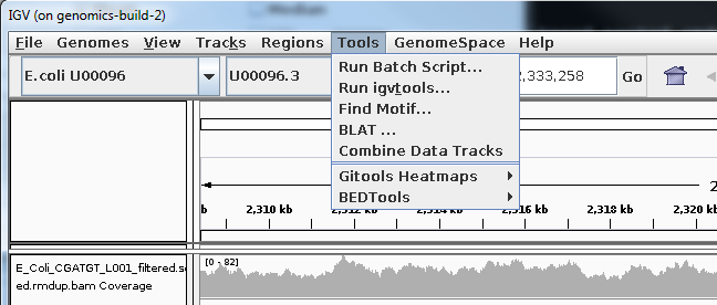
Now load the BAM alignment file in the Input field and click Run:

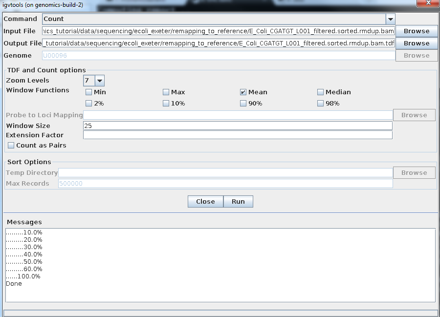
Once completed, you can load this TDF file as by:

Select File -> Load from file

Select the TDF file you have just created.

You should then see the extra coverage track which remains visible even after you zoom out.+

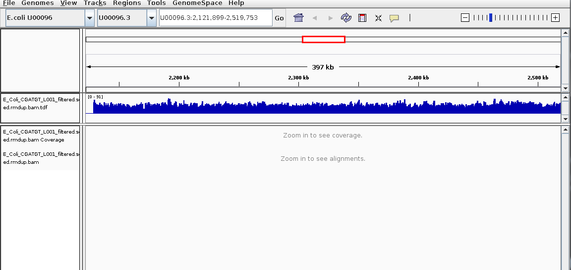
Again try to use the QualiMap report to give you an idea. What is this region? Is there a gene close-by? What do you think this is? (Think about repetitive sequences, what does BWA do if a region in the genome has been duplicated)

Task 21: Identify SNPs and Indels manually

• Can you find any SNPs?
• Which genes (if any) are they in?
• How reliable do they look? (Hint: look at the number of reads mapping, their orientation - which strand they are on and how bright the base calls are).

Zoom in to maximum magnification at the site of the SNP. Can you determine whether a SNP results in a synonymous (i.e. silent) or non-synonymous change in the amino acid? Can you use PDB (http://www.rcsb.org/pdb/home/home.do) or other resources to determine whether or not this occurs in a catalytic site or other functionally crucial region? (Note this may not always be possible).

What effect do you think this would have on the cell?

Here are some regions where there are differences in the organism sequenced and the reference: Can you interpret what has happened to the genome of our strain? Try to work out what is going on yourself before looking at the comment

Paste each of the genomic locations in this box and click go

U00096.3:2,108,392-2,133,153

U00096.3:3,662,049-3,663,291

U00096.3:4,296,249-4,296,510

U00096.3:565,965-566,489

Region U00096.3:2,108,392-2,133,153

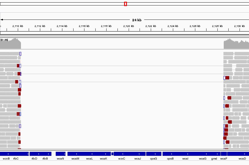
This area corresponds to the drop in coverage identified by Qualimap. It looks like a fairly large region of about 17K bases which was present in the reference and is missing from our sequenced genome. It looks like about 12 genes from the reference strain are not present in our strain - it this real or an artefact?

Well it is pretty conclusive we have coverage of about 60X either side of the deletion and nothing at all within. There are nice clean edges to the start and end of the deletion. We also have paired reads which span the deletion. This is exactly what you would expect if the two regions of coverage were actually joined together.

Region U00096.3:3,662,049-3,663,291

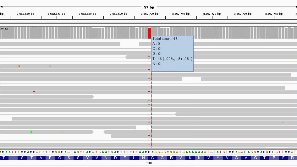
Zoom right in until you can see the reference sequence and protein sequence at the bottom of the display.

The first thing to note is that only discrepancies with respect to the reference are shown. If a read is entirely the same as its reference, it will appear entirely grey. Blue and red blocks indicate the presence of an ‘abnormal’ distance between paired-end reads. Note that unless this is consistent across most of the reads at a given position, it is not significant.

Here we have a C->T SNP. This changes the codon from CAG->TAG (remember to check what strand the gene is on this one is on the forward strand, if it was on the reverse strand you would have to take the reverse complement of the codon to interpret the amino acid it codes for.) and results in a Gln->Stop mutation in the final protein product which is very likely to change the effect of the protein product.

Hover over the gene to get some more information from the annotation…

Since it is a drug resistance protein it could be very significant.

One additional check is that the SNPs occur when reading the forward strand. We can check this by looking at the direction of the grey reads,or by hovering over the coverage graph - see previous diagram. We can see that approximately half of the bases reporting the C->T mutation occur in read 1 (forward arrow), and half in read 2 (reverse arrow). This adds confidence to the base-call as it reduces the likelihood of this SNP being the result of a PCR duplication error.

Note that sequencing errors in Illumina data are quite common (look at the odd bases showing up in the screen above. We rely on depth of sequencing to average out these errors. This is why people often mention that a minimum median coverage of 20-30x across the genome is required for accurate SNP-calling with Illumina data. This is not necessarily true for simple organisms such as prokaryotes, but for diploid and polyploid organisms it becomes important because each position may have one, two or many alleles changed.

Region U00096.3:4,296,249-4,296,510

Much the same guidelines apply for indels as they do for SNPs. Here we have an insertion of two bases CG in our sample compared to the reference. Again, we can see how much confidence we have that the insertion is real by checking that the indel is found on both read 1 and read 2 and on both strands.

The insertion is signified by the presence of a purple bar. Hover your mouse over it to get more details as below

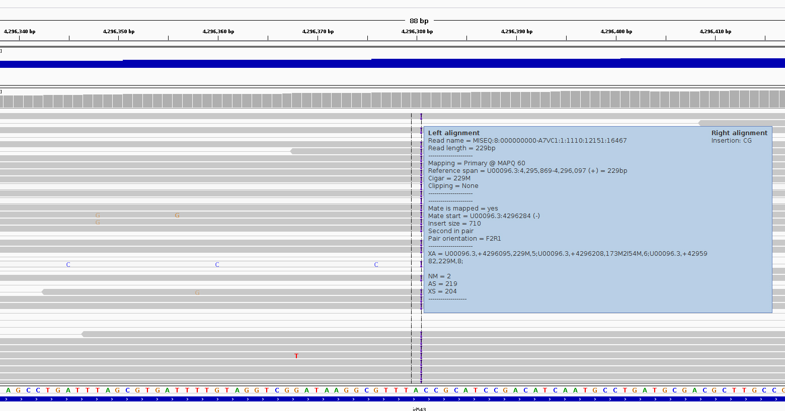
We can hover our mouse over the reference sequence to get details of the gene. We can see that it occurs in a repeat region and is unlikely to have very significant effects.

One can research the effect that a SNP or Indel may have by finding the relevant gene at http://www.uniprot.org (or google ‘mdtF uniprot’ in the previous case).

It should be clear from this quick exercise that trying to work out where SNPs and Indels are manually is a fairly tedious process if there are many mutations. As such, the next section will look at how to obtain spread-sheet friendly summary details of these.

Region U00096.3:565,965-566,489

This last region is more complex try to understand what genomic mutation could account for this pattern - discuss with a colleague or an instructor.

Recap: SNP/Indel identification

• Only changes from the reference sequence are displayed in IGV
• Genuine SNPs/Indels should be present on both read 1 and read 2
• Genuine SNPs/Indels should be present on both strand
• Genuine SNPs/Indels should be supported by a good (i.e. 20-30x) depth of coverage
• Very important mutations (i.e. ones relied upon in a paper) should be confirmed e.g. using PCR.

Task 22: Identify SNPs and Indels using automated variant callers

Viewing alignments is useful when convincing yourself or others that a particular mutation is real rather than an artefact and for getting a feel for short read sequencing datasets. However, if we want to quickly and easily find variants we need to be able to generate lists of variants, in which gene they occur (if any) and what effect they have. We also need to know which (if any) genes are missing (i.e. have zero coverage).

To call variants we can use a number of packages (e.g. VarScan, GATK). However here, we will show you how to use the bcftools package which comes with samtools. First we need to generate a pileup file which contains only locations with the variants and pass this to bcftools.

Make sure you are in the correct directory.
cd ~/workshop_materials/genomics_tutorial/data/sequencing/ecoli_exeter/remapping_to_reference
and type the following:

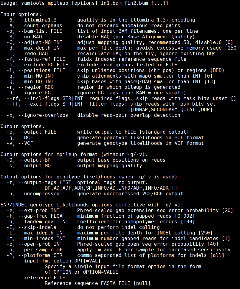
samtools mpileup

You should see a screen similar to the following

If you are running this on datasets with large numbers of datasets with limited coverage where recombination is a factor, you can obtain increased sensitivity by passing all the BAM files to the variant caller simultaneously (hence the multiple BAM file options in samtools).

Type the following:

samtools mpileup -v -u -P Illumina --reference ~/workshop_materials/genomics_tutorial/data/reference/U00096/U00096.fna E_Coli_CGATGT_L001_filtered.sorted.rmdup.bam > var.raw.vcf

This may take 10 minutes or so and will generate a VCF file containing the raw unfiltered variant calls for each position in the genome. Note that we are asking samtools mpileup to generate uncompressed VCF output with the -v and -u options. -P tells samtools it is dealing with Illumina data so that it can apply to the correct model to help account for mis-calls or indels.

This output by itself is not useful to us since it contains information on each position in the genome. So lets use the sister package of samtools, called bcftools to call what it thinks are the variant sites:

bcftools --help

bcftools call -c -v --ploidy 1 -O v -o var.called.vcf var.raw.vcf

Note that we are asking bcftools to call using assuming a ploidy of 1 and to output only the variant sites in VCF format. Using grep we can count how many sites were identified as being variant sites (i.e. sites with a potential mutation). We ask grep not to count lines beginning with a comment (#).

grep -v -c "^#" var.called.vcf

You should find 320 or so sites.

Now we just need to filter this a bit further to ensure we only retain regions where we have >90% allele frequency:

vcftools --min-alleles 2 --max-alleles 2 --non-ref-af 0.9 --vcf var.called.vcf --recode --out var.called.filt

(the output will be called var.called.filt.recode.vcf)

Once complete, view the file using the ‘more’ command. You should see something similar to: (lines beginning with # are just comment lines explaining the output)

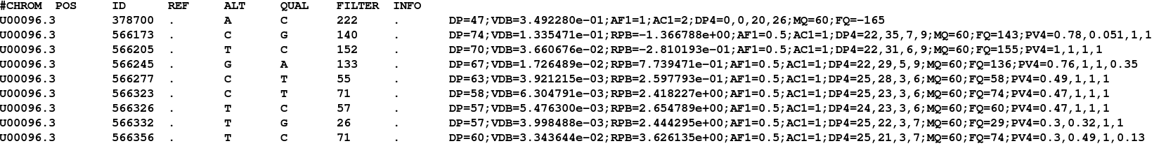
You can see the chromosome, position, reference and alternate allele as well as a quality score for the SNP. This is a VCF file (Variant Call File). This is a standard developed for the 1000 genomes project.

The full specification is given at http://samtools.github.io/hts-specs/VCFv4.2.pdf

The lines starting DP and INDEL contain various details concerning the variants. For haploid organisms, most of these details are not necessary.

This forms our definitive list of variants for this sample.

Take a look at some of the variants we just excluded, was it justified? Remember there is no filter that can keep all the correct variants and remove all the dubious!

You can load the VCF file to IGV:

Task 23: Compare the variants found using this method to those you found in the manual section

Can you see any variants which may have been missed? Often variants within a few bp of indels are filtered out as they could be spurious SNPs thrown up by a poor alignment. This is especially the case if you use non-gapped aligners such as Bowtie.

Task 24 locating genes which are missing compared to the reference

We can use a command from the BEDTools package (http://bedtools.readthedocs.org/en/latest/) to identify annotated genes which are not covered by reads across their full length.

Type the following on one line:

coverageBed -a ~/workshop_materials/genomics_tutorial/data/reference/U00096/U00096.gff -b E_Coli_CGATGT_L001_filtered.sorted.rmdup.bam > gene_coverage.txt

This should only take a minute or so. The output contains one row per annotated gene - the last column contains the proportion of the gene that is covered but reads from our sequencing. 1.00 means the gene is 100% covered and 0.00 means no coverage.

If we sort by this column we can see which genes are missing (N.B. -k 13 means sort by the 13th column, replace the 13 by whatever the final column number is in your file):

sort -t$'\t' -g -k 13 gene_coverage.txt | more

There is another region of about 10kb which is absent from out sequences - can you find it in IGV?

Task 25: Determine the effect of variants

So far we have found a number of genes missing from this strain of E.coli which obviously could have a phenotypic effect. Let’s now take a closer look at the variants. We’d like to obtain a list of genes in which these variants occur and whether they result in amino acid changes.

To do this we’ll use a custom perl script developed by David Studholme and Konrad Paszkiewicz.

We’ll just need the reference annotation, sequence and the VCF file containing the SNPs.

snp_comparator.pl 10 ~/workshop_materials/genomics_tutorial/data/reference/U00096/U00096.fna ~/workshop_materials/genomics_tutorial/data/reference/U00096/U00096.gff var.called.filt.recode.vcf  > snp_report.txt

You will see lots of warnings about ‘Use of uninitialized value $gene_name - you can ignore these.

This program takes the information from the reference sequence and annotation, and the VCF SNP files and determines whether the variant occurs within a gene, and if so the effect of each mutation.

Once complete, view the snp_report.txt file.

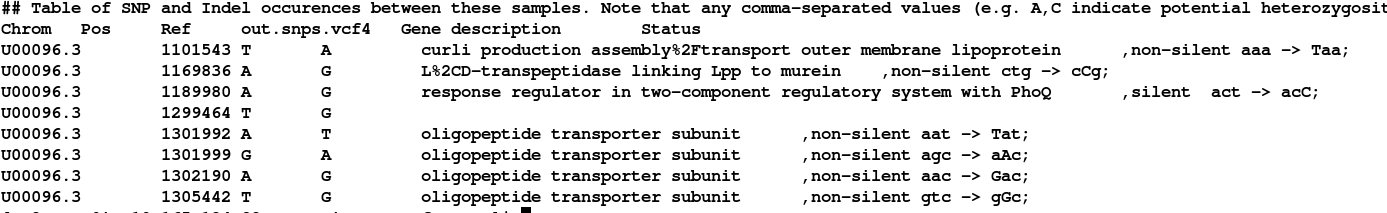
In later workshops we will see how we can use this program to compare results between different strains.

You can also use tools such as SNPEff to evaluate the effect of variants (http://snpeff.sourceforge.net/index.html)

Task 26: Check each variant in IGV

**N.B. If a variant doesn’t seem to match what the snp_report file says, check the reverse reading frames.

That concludes the first part of the course. You have successfully, QC’d, filtered, remapped and analysed a whole bacterial genome! Well done!

In the next instalment we will be looking at how to extract and assemble unmapped reads. This will enable us to look at material which may be present in the strain of interest but not in the reference sequence.

Part 3. Unmapped Read Assembly

Background

In this section of the workshop we will continue the analysis of a strain of E.coli. In the previous section we cleaned our data, checked QC metrics, mapped our data and obtained a list of variants and an overview of any missing regions.

Now, we will examine those reads which did not map to the reference genome. We want to know what these sequences represent. Are they novel genes, plasmids or just contamination?

To do this we will extract unmapped reads, evaluate their quality, prepare them for de novo assembly, assemble them using SPAdes, generate assembly statistics and then produce some annotation via Pfam, BLAST and RAST.

Extraction and QC of unmapped reads

Task 1: Extract the unmapped reads

First of all make sure you are in the directory
~/workshop_materials/genomics_tutorial/data/sequencing/ecoli_exeter
(hint: use the cd command).

Then create a directory called unmapped_assembly in which we will do our de novo assembly and analysis.

mkdir unmapped_assembly
cd unmapped_assembly/

Now we will use the bam2fastq program (http://gsl.hudsonalpha.org/information/software/bam2fastq) to extract from the BAM file just those reads which did NOT map to the reference genome. The bam2fastq program has a number of options, most of which are self-explanatory. Type (all on one line):

bam2fastq --no-aligned -o unaligned#.fastq ../remapping_to_reference/E_Coli_CGATGT_L001_filtered.sorted.rmdup.bam

The –no-aligned option means only extract reads which did not align. The -o unaligned# means dump read 1 into a file called unaligned_1.fastq and read 2 into a file unaligned_2.fastq. Below we can see that the program has successfully created the two files.

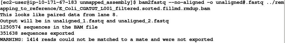
Note that some reads were singletons (i.e. one read mapped to the reference, but the other did not). These will not be included in this analysis.

Task 2: Check the extraction looks correct Check that the number of entries in both fastq files is the same. Also check that the last few entries in the read 1 and read 2 files have the same header (i.e. that they have been correctly paired).

Task 3: Evaluate QC of unmapped reads

Use the fastqc program to look at the statistics and QC for the unaligned_1.fastq and unaligned_2.fastq files.

Do these look reasonably good? Remember, some reads will fail to map to the reference because they are poor quality, so the average scores will be lower than the initial fastqc report we did in the remapping workshop. The aim here is to see if it looks as though there are reads of reasonable quality which did not map.

Assuming these reads look ok, we will proceed with preparing them for de novo assembly.

De-novo assembly

de-novo* is a Latin expression meaning “from the beginning,” “afresh,” “anew,” “beginning again.” when we perform a de novo assembly we try to reconstruct a genome or part of the genome from our reads without making any prior assumptions (in contrast to remapping where we compare out reads to what we think is a close reference sequence).

The advantage is that is that de novo assembly can reveal completely novel results, identify horizontal gene transfer events for example. The disadvantage is that it is difficult to get a good assembly from short reads and it can be prone to misleading results due to contamination and mis-assembly.

Task 4: Learn more about de novo assemblers

To understand more about de-novo assemblers, read the technical note at: https://www.illumina.com/Documents/products/technotes/technote_denovo_assembly_ecoli.pdf

N.B. You will also learn more in the next section so don’t worry if it doesn’t all make sense immediately. You should however understand the idea of the k-mer and broadly how the assembly is built up from them.

Task 5: Generate the assembly.

We will be using an assembler called SPAdes (http://cab.spbu.ru/software/spades/). It generally performs pretty well with a variety of genomes. It can also incorporate longer reads produced from PacBio sequencers that we will use later in the course.

One big advantage is that it is not just a pure assembler - it is a suite of programs that prepare the reads you have, assembles them and then refines the assembly.

SPAdes runs the modules that are required for a particular dataset and it produces the assembly with a minimum of preparation and parameter selection - making it very straightforward to produce a decent assembly. As with everything in bio-informatics you should try to assess the results critically and understand the implications for further analysis.

Let’s start the assembler because it takes a few minutes to run.

spades.py -k 21,33,55,77,99,127 --careful -o spades_assembly -1 unaligned_1.fastq -2 unaligned_2.fastq

We are telling it to run the SPAdes assembly pipeline with a range of k-mer sizes (-k); specifying –careful tells it to run a mismatch correction algorithm to reduce the number of errors; put the output in the spades_assembly directory and the reads to assemble.

Just because SPAdes does a lot for you does not mean you should not try to understand the process.

Have a read of this: http://thegenomefactory.blogspot.co.uk/2013/08/how-spades-differs-from-velvet.html It is a discussion of how SPAdes differs from Velvet another widely used assembler, it explains the overall process nicely:

• Read error correction based on k-mer frequencies using BayesHammer
• De Bruijn graph assembly at multiple k-mer sizes, not just a single fixed one.
• Merging of different k-mer assemblies (good for varying coverage)
• Scaffolding of contigs from paired end/mate pair reads
• Repeat resolution from paired end/mate pair data using rectangle graphs
• Contig error correction based on aligning the original reads with BWA back to contigs.

Try to understand the steps in the context of the whole picture:
Can you explain why depth of coverage and error correction of reads becomes more important as k-mer length increases?

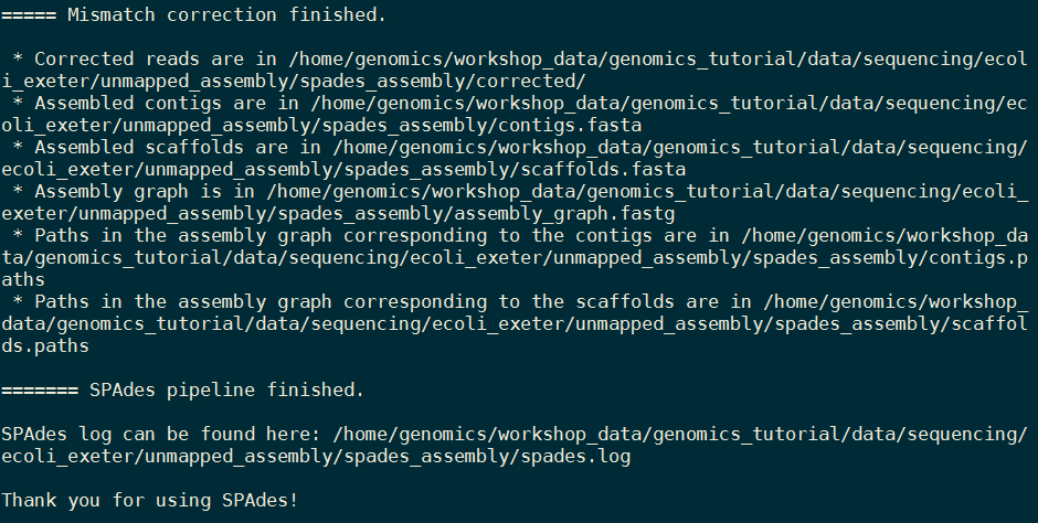
When the assembly is complete: Change to the spades_assembly directory (use cd) and look at the output.

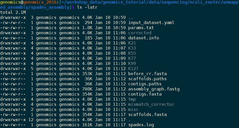
Let’s take a look at some of the more important content.

• params.txt - a summary of the parameters used for assembly it is useful so you can repeat the exact analysis performed, or can remember you setting when you want to publish the genome.
• contigs.fasta - the final results of the assembly in fasta format.
• scaffolds.fasta - the final results after scaffolding (which means using paired end information to join contigs together with gaps). In this case the files are identical, probably because the sum of the lengths of our paired reads is not much smaller than our insert size (there are very few large gaps between reads).
• assembly_graph.fastg SPAdes assembly graph in FASTG format - this is a slightly different format that contains more information than fasta - for example it can contain alternative alleles in diploid assemblies. We don’t need it here, but see http://fastg.sourceforge.net/FASTG_Spec_v1.00.pdf if you might be working with diploid organisms. You can use the Bandage (http://rrwick.github.io/Bandage/) to view this file.

Task 6: Assessment of the assembly

We will use QUAST (http://quast.sourceforge.net/quast) to generate some statistics on the assembly (in the spades_assembly directory)

cd spades_assembly
quast.py --output-dir quast contigs.fasta

This will create a directory called quast and create some statistics on the assembly you produced.

cat quast/report.txt

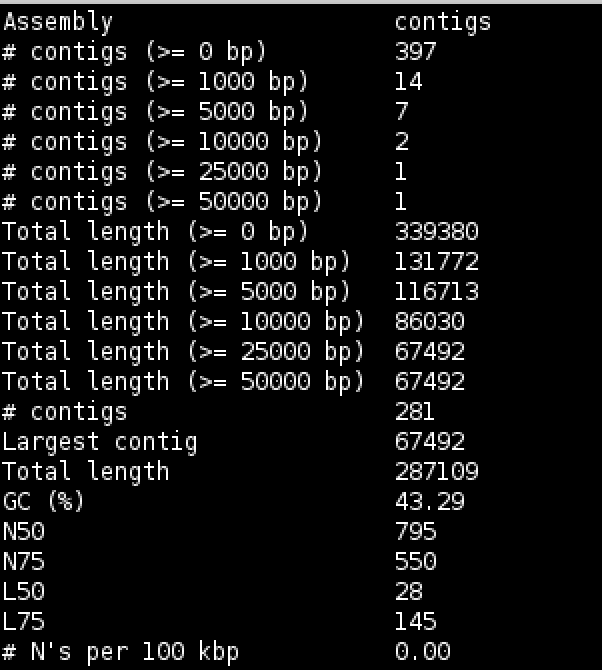
Try to interpret the information in the light of what we were trying to do. Because we are assembling unaligned reads we are not expecting a whole chromosome to pop out. We are expecting bits of our strain that does not exist in the reference we aligned against; possibly some contamination; various small contigs made up of reads that didn’t quite align to our reference.

The N50 and L50 measures are very important in a normal assembly and we will visit them later, they are not really relevant to this assembly.

You will notice that we have 1 contig 30-60kb long - what do you think this might be? And 12 other contigs longer than 1kb. We should find out what this is.

Now that we have assembled the reads and have a feel for how much (or in this case, how little) data we have, we can set about analysing it. By analysing, we mean identifying which genes are present, which organism they are from and whether they form part of the main chromosome or are an independent unit (e.g. plasmid).

We are going to take a 3-prong approach. The first will simply search the nucleotide sequences of the contigs against the NCBI non-redundant database. This will enable us to identify the species to which a given contig matches best (or most closely). The second will call open reading frames within the contigs and search those against the Swissprot database of manually curated (i.e. high quality) annotated protein sequences. Finally, we will search the open reading frames against the Pfam database of protein families (http://pfam.xfam.org/).

Why not just search the NCBI blast database? Well, remember nearly all of our biological knowledge is based on homology - if two proteins are similar they probably share an evolutionary history and may thus share functional characteristics. Metrics to define whether two sequences are homologous are notoriously difficult to define accurately. If two sequences share 90% sequence identity over their length, you can be pretty sure they are homologous. If they share 2% they probably aren’t. But what if they share 30%? This is the notorious twilight zone of 20-30% sequence identity where it is very difficult to judge whether two proteins are homologous based on sequence alone.

To help overcome this searching more subtle signatures may help - this is where Pfam comes in. Pfam is a database which contains protein families identified by particular signatures or patterns in their protein sequence. These signatures are modeled by Hidden Markov Models (HMMs) and used to search query sequences. These can provide a high level annotation where BLAST might otherwise fail. It also has the advantage of being much faster than BLAST.

Task 7: Search contigs against NCBI non-redundant database

Firstly we can filter out low coverage and very short contigs using a perl script: filter_low_coverage_contigs.pl < contigs.fasta > contigs.goodcov.fasta

The following command executes a nucleotide BLAST search (blastn) of the sequences in the contigs.fa file against the non-redundant database. As this takes a long time to run the results have been precomputed and are available in
~/workshop_materials/genomics_tutorial/data/sequencing/ecoli_exeter/blast_precompute/unmapped_reads/

blastn -db ~/workshop_materials/genomics_tutorial/db/blast/nt -query contigs.goodcov.fasta -evalue 1e-06 -num_threads 8 -show_gis -num_alignments 10 -num_descriptions 10 -out contigs.fasta.blastn

There are a lot of options in this command, let’s go through them

• -db is the prepared blast database to search

• evalue apply an e-value (expectation value) (http://www.ncbi.nlm.nih.gov/BLAST/tutorial/Altschul-1.html) cutoff of 1e-06 to limit ourselves to statistically significant hits (i.e. in this case 1 in 1 million likelihood of a hit to a database of this size by a sequence of this length).

• -num_alignments and -num_descriptions flags tell blastn to only display the top 10 results for each hit.
• -num_threads that it should use 8 CPU cores \
• -show_gis that it should include general identifier (GI) numbers in the output.
• -out file in which to place the output.

There is lots of information on running blast from the command line at http://www.ncbi.nlm.nih.gov/books/NBK1763/

N.B. GI (GeneInfo Identifiers) are being phased out by NCBI so future versions of Blast and NCBI databases will not support the -show_gis option and may break some down-stream tools such as KronaTools and other databases.

Open the results file pluma contigs.fasta.blastn

BLASTN 2.2.31+


Reference: Zheng Zhang, Scott Schwartz, Lukas Wagner, and Webb
Miller (2000), "A greedy algorithm for aligning DNA sequences", J
Comput Biol 2000; 7(1-2):203-14.



Database: Nucleotide collection (nt)
           29,442,065 sequences; 84,823,117,434 total letters



Query= NODE_1_length_67364_cov_602.091

Length=67364
                                                                      Score     E
Sequences producing significant alignments:                          (Bits)  Value

gi|664682453|gb|CP008801.1|  Escherichia coli KLY, complete genome    86309   0.0  
gi|8918823|dbj|AP001918.1|  Escherichia coli K-12 plasmid F DNA, ...  86272   0.0  
gi|619497957|gb|KJ170699.1|  Escherichia coli strain K-12 plasmid...  65330   0.0  
gi|665821556|gb|KJ484626.1|  Escherichia coli plasmid pH2332-166,...  65302   0.0  
gi|665821958|gb|KJ484628.1|  Escherichia coli plasmid pH2291-144,...  65213   0.0  
gi|28629230|gb|AF550679.1|  Escherichia coli plasmid p1658/97, co...  64591   0.0  
gi|4874241|gb|U01159.2|  Escherichia coli F sex factor transfer r...  61474   0.0  
gi|665822931|gb|KJ484636.1|  Escherichia coli plasmid pC59-153, c...  41227   0.0  
gi|301130432|gb|CP002090.1|  Salmonella enterica subsp. enterica ...  41026   0.0  
gi|301130304|gb|CP002089.1|  Salmonella enterica subsp. enterica ...  41026   0.0  

. . .

SPAdes names the contigs by increasing size, so ‘NODE_1’ is the longest contig.

There are a number of good hits; notice from the contig header line that the average coverage is >500 and the coverage of our genome was around 50 - does this give you a clue to what it is?

Task 8: Obtain open reading frames

The first task is to call open reading frames within the contigs. These are designated by canonical start and stop codons and are usually identified by searching for regions free of stop codons. We will use the EMBOSS package program getorf to call these.

We will use codon table 11 which defines the bacterial codon usage table (http://www.ncbi.nlm.nih.gov/Taxonomy/Utils/wprintgc.cgi) and state that the sequences we are dealing with are not circular (only the 67k contig is long enough!). We will also restrict the ORFs to just those sequences longer than 300 nucleotides (i.e. 100 amino acids). We will store the results in file contigs.orf.fa.

getorf -table 11 -circular N -minsize 300 -sequence contigs.goodcov.fasta -outseq contigs.orf.fasta

If we look at the output file we can see that it is a FASTA formatted file containing the name of the contig on which the ORF occurs, followed by an underscore and a number (e.g. _1) to indicate the number of the ORF on that contig. The numbers in square brackets indicate the start and end position of the ORF on the contig (i.e. in nucleotide space). So the first ORF occurs on NODE 9 and is between position 934 and 1494. The third ORF occurs between positions 2400 and 2047 on the reverse strand. This is a relatively short peptide sequence and is unlikely to be a genuine peptide.

Also note that many ORFs do not start with a Methionine. This is because by default the getorf program calls ORFs between stop codons rather than start and stop codons. Primarily this is to avoid spurious ORFs due to Met residues within a protein sequence and to ensure untranslated regions are captured.

>NODE_9_length_3631_cov_29.6618_ID_17_1 [934 - 1494]  \
TERFEVSEINSQALREAAEQAMHDDWGFDADLFHELVTPSIVLELLDERERNQQYIKRRD
QENEDIALTVGKLRVELETAKSKLNEQREYYEGVISDGSKRIAKLESNEVREDGNQFLVV
RHPGKTPVIKHCTGDLEEFLRQLIEQDPLVTIDIITHRYYGVGGQWVQDAGEYLHMMSDA
GIRIKGE
>NODE_9_length_3631_cov_29.6618_ID_17_2 [2450 - 3529]  \
RGSEMGRRRSHERRDLPPNLYIRNNGYYCYRDPRTGKEFGLGRDRRIAITEAIQANIELF
SGHKHKPLTARINSDNSVTLHSWLDRYEKILASRGIKQKTLINYMSKIKAIRRGLPDAPL
EDITTKEIAAMLNGYIDEGKAASAKLIRSTLSDAFREAIAEGHITTNHVAATRAAKSEVR
RSRLTADEYLKIYQAAESSPCWLRLAMELAVVTGQRVGDLCEMKWSDIVDGYLYVEQSKT
GVKIAIPTALHIDALGISMKETLDKCKEILGGETIIASTRREPLSSGTVSRYFMRARKAS
GLSFEGDPPTFHELRSLSARLYEKQISDKFAQHLLGHKSDTMASQYRDDRGREWDKIEIK
>NODE_9_length_3631_cov_29.6618_ID_17_3 [2400 - 2047] (REVERSE
SENSE)  
FVEQILSSILNRRWEYPAFPNPSTNCFKASWTSLACVPLLKCQVHRKVSAITRKKKPPSG
GLVFFQFFNSNIGYVCMCYLRPYHPVVVAVVDVLRFDNSVEWLSIPFSCDSEVHLSSP

Task 9: Search open reading frames against NCBI non-redundant database

The first thing we can do with these open reading frames is to search them against the NCBI non-redundant database of protein sequences to see what they may match.

First reduce the number of orfs so that we have a manageable number - this small perl program selects 10% of the orfs.

reduce_fasta_10x.pl < contigs.orf.fasta > contigs.orf.small.fasta

Then you would type (all on one line). HOWEVER this could take a while, therefore the results have been precomputed in ~/workshop_materials/genomics_tutorial/data/sequencing/ecoli_exeter/blast_precompute/unmapped_reads/

blastp -db ~/workshop_materials/genomics_tutorial/db/blast/nr -query contigs.orf.small.fasta -evalue 1e-06 -num_threads 2 -show_gis -num_alignments 10 -num_descriptions 10 -out contigs.orf.blastp

Task 10: Review the BLAST format

Open the results file with pluma and search for plasmid in the text. You should find a number of hits to plasmid related proteins - one example is below - can you find any others? (Remember we only checked 10% of the orfs we found). This evidence is not conclusive, but combined with the high coverage over, it is starting to look like this contig is a plasmid.

Query= NODE_1_length_67364_cov_602.091_17 [9087 - 9569]

Length=161
                                                                      Score     E
Sequences producing significant alignments:                          (Bits)  Value

gi|553349257|gb|ESA76469.1|  Protein PsiB                             322     5e-110
gi|503044320|ref|WP_013279296.1|  plasmid SOS inhibition protein B    320     2e-109
gi|324006232|gb|EGB75451.1|  plasmid SOS inhibition protein (PsiB)    310     2e-105
gi|300355538|gb|EFJ71408.1|  plasmid SOS inhibition protein (PsiB)    308     5e-105
gi|324010272|gb|EGB79491.1|  plasmid SOS inhibition protein (PsiB)    305     2e-103
gi|505582716|ref|WP_015675404.1|  recombinase                         300     1e-101
gi|446768672|ref|WP_000845928.1|  recombinase                         299     2e-101
gi|301073353|gb|EFK88159.1|  Protein PsiB                             300     2e-101
gi|446768671|ref|WP_000845927.1|  recombinase                         297     1e-100
gi|446610348|ref|WP_000687694.1|  recombinase                         297     1e-100

Task 11: Check that the contigs do not appear in the reference sequence

In theory, the unmapped reads used to generate the contigs should not assemble into something which will map against the genome. However, it is always possible (especially with more complex genomes), that this might happen. To double-check move back to the folder containing the contigs.goodcov.fasta:

blastn -subject ~/workshop_materials/genomics_tutorial/data/reference/U00096/U00096.fna -query contigs.goodcov.fasta | more

Here we use the BLAST+ package in a different mode to compare two sequences against each other. Unlike the previous examples where we have searched against a database of sequences, here we are doing a simple search of the contigs against the reference genome we are using. Scroll down a little…

Query= NODE_18_length_917_cov_10.7608

Length=917

Subject= U00096.3

Length=4641652


 Score = 193 bits (104),  Expect = 3e-49
 Identities = 186/227 (82%), Gaps = 0/227 (0%)
 Strand=Plus/Minus

Query  624      GCCTTTGGCGTTGCAGCAAGCGTTTCAGACGTGCTGTTGGTTGCACTGCTGAGCTGCACT  683
                |||||||||||||| || |||||||||||||| |||||||| |||||||||||||| |||
Sbjct  1430511  GCCTTTGGCGTTGCCGCCAGCGTTTCAGACGTACTGTTGGTCGCACTGCTGAGCTGTACT  1430452

Query  684      ATCCCCTTTCTCGTTGTGTCCGCATCCTCAAGCGCGACAGCTGAAGCTATATCTTCTGCA  743
                ||||||||| |||| ||    |||||||||||||| || || || || ||||| ||||| 
Sbjct  1430451  ATCCCCTTTTTCGTCGTACTTGCATCCTCAAGCGCCACGGCGGATGCAATATCCTCTGCC  1430392

You can see that some of the contigs that have been assembled hit the reference sequence. In the record above the evalue is 3e-49 which is massively significant; however, the evalue is calculated as the chance of a hit this close against a random sequence of the same size. Since our subject sequence is now very small and we know it is related to our strain it is not surprising that there are some hits. We are concerned about whole contigs that map closely to the reference genome.

Task 12: Run open reading frames through pfam_scan

Pfam is a database of protein families. They are grouped together using a number of criteria based on their function. For more information read http://en.wikipedia.org/wiki/Pfam.

Pfam is grouped into several databases depending on the level of curation. Pfam-A is high-quality manual curation and consists of around 12,500 families. Pfam-B is full of automated predictions which may be informative but should not be relied upon without additional evidence. Pfam will also search for signatures of active-sites if you specify the correct flag.

Here we want to search the Pfam database of Hidden Markov Models to see which protein families are contained within this contig. You’ll notice that this runs considerably faster than BLAST. Here we search using the contigs.orf.fa file against the Pfam databases ~/genomics_tutorial/db/pfam/ and output the results to contigs.orf.pfam. We’ll use 2 CPU cores for the search and state that we want to search PfamB entries as well as active site residues.

This step might take about 30 minutes. So you can get a coffee in the meantime.

pfam_scan.pl -fasta contigs.orf.fasta -dir ~/workshop_materials/genomics_tutorial/db/pfam/ -outfile contigs.orf.pfam -cpu 2 -pfamB -as

View the output using pluma:

Search for NODE_9 (for example).

NODE_9_length_3631_cov_31.6458_1         7    106      7    106 PF13935.1   Ead_Ea22          Family     1   139   139    103.8     9e-30   1 No_clan  
NODE_9_length_3631_cov_31.6458_1        77    113     77    126 PB009353    Pfam-B_9353       Pfam-B     1    37    82     53.4   2.8e-14  NA NA      
NODE_9_length_3631_cov_31.6458_2         5     74      5     75 PF09003.5   Phage_integ_N     Domain     1    75    76     89.5     8e-26   1 CL0081   
NODE_9_length_3631_cov_31.6458_2        85    162     84    162 PF02899.12  Phage_int_SAM_1   Domain     2    84    84     24.1     3e-05   1 CL0469   
NODE_9_length_3631_cov_31.6458_2       183    349    182    353 PF00589.17  Phage_integrase   Family     2   169   173    115.1   2.6e-33   1 CL0382   predicted_active_site[239,312,216,346,337,315]
NODE_9_length_3631_cov_31.6458_3        53    115     48    117 PB009641    Pfam-B_9641       Pfam-B    50   112   168     23.3   6.7e-05  NA NA      

The 8th column shows the type of entry that was hit in the pfam database.

Go to http://pfam.xfam.org/ and enter the Pfam domain in the search box.
Let’s take a look at Pfam domain Phage_integ_N

There are a lot of hits to phage domains and domains that manipulate DNA. You might expect this as these sequences have presumably been incorporated into our strain since it diverged from the reference.

Also look at domains (the most specific type of hit) from our large contig NODE_1_….. is there any evidence for it being a plasmid?

The Pfam-B matches do not tell you much that is useful.

Examine one or two more domains from your results file - is there anything interesting?

Analysing the results in RAST

By now you should be able to see that analysing results for de novo assembled reads of any sort can be difficult and time-consuming. Bear in mind that we have only been faced with a single contig of 3kb. Quite often you may find yourself dealing with hundreds, if not thousands of contigs. Some will be a few 100kb long. Others may only be 200-300bp. How should we go about analysing these in a more efficient manner? There are a number of options here.

For eukaryotes I would suggest looking at MAKER (http://www.yandell-lab.org/software/maker.html).

For prokaryotes the situation is somewhat easier and we can use a web-based service known as RAST. This is not the only service (Xbase is another), but it is one of the most commonly used.

RAST is a website where you upload the results of your de novo assembly and RAST will attempt to provide annotation in commonly used GFF and Genbank formats. This can be used to load up the annotation in Artemis or Apollo. Alternatively RAST has its own in-built viewer.

Task 13 (Optional) Log in to RAST

Within your instance, go to http://rast.nmpdr.org/ Log-in with the details RAST provided to you before you started this series of workshops. If you do not have one, you may need to wait several days for your login to be issued by RAST. Please skip ahead and come back to this section.

Task 14 (Optional) Upload the assembled contigs and annotate using RAST Click on Your jobs->Upload New Job

Upload the contigs.fasta file obtained by the de novo assembly of unmapped reads. Click on ‘Use this data’ and go to step 2.

We know this is an E.coli genome so we can enter 562 as the Taxonomy ID and click on ‘Fill in form based on NCBI taxonomy-ID’. If you’re dealing with a different organism, be sure to change this number. RAST will automatically split any scaffolds (i.e. contigs with bits missing in the middle - denoted by Ns). Then click ‘Use this data and go to step 3’.

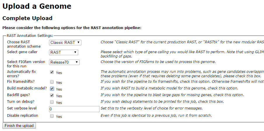
Replicate the settings above and click on ‘Finish the upload’.

Your job may take several hours to run. In the meantime, proceed to the next workshop and come back to this later.

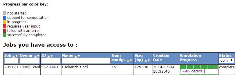
Once complete, RAST should email you a message. You can then view the results or download them in standardized formats (e.g. GFF3, Genbank, EMBL etc).

On the start page click on view details for your annotation

You will get a summary of the sequence you uploaded and you have the ability to download the annotations to your computer.

Download the GFF3 annotation and open it in a text editor

##gff-version 3 NODE_10_length_3324_cov_22.7003_ID_19 FIG CDS 249 1163 . 0 ID=fig|562.4461.peg.1;Name=FIG010773: NAD-dependent epimerase/dehydratase

note: your output may be different. Scan down the list of annotations do any themes stand out?

Click on ‘Browse annotated genome in SEED viewer’

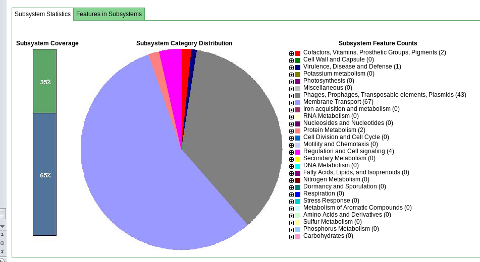
This gives you a hierarchical view of the subsystems.

Browse the rest of the RAST server and get a feel for the possibilities the platform may offer you.

When you’re ready, move on to (or back to) the de novo assembly part of the workshop.

Part 4. De-novo Assembly

Introduction:

In this section of the workshop we will continue the analysis of a strain of E.coli. In the previous section we extracted those reads which did not map to the reference genome and assembled them. However, it is often necessary to be able to perform a de-novo assembly of a genome. In this case, rather than doing any remapping, we will start with the filtered reads we obtained in part 3 of the workshop.

To do this we will a program called SPAdes to try to get the best possible assembly for a given genome. We will then generate assembly statistics and then produce some annotation via Pfam and BLAST.

Task 1: Start the Assembly

The assembly takes so the results have been pre-computed for you and are available in the directory

~/workshop_materials/genomics_tutorial/data/sequencing/ecoli_exeter/denovo_assembly

If you were to run the command it would be as follows:

spades.py -o denovo_assembly_rerun -1 E_Coli_CGATGT_L001_R1_001.filtered.fastq -2 E_Coli_CGATGT_L001_R2_001.filtered.fastq

This will create a directory called denovo_assembly_rerun to hold the results.

**Assembly theory **

We are using SPAdes (http://cab.spbu.ru/software/spades/) to perform our assembly. It is a de Bruijn graph based assembler, similar to other short read assemblers like velvet (https://www.ebi.ac.uk/~zerbino/velvet/). The advantage of SPAdes is that it does lot of error correction and checking before and after the assembly which improve the final result. A downside of SPAdes is that it was designed for assembling reads from a single cell and although it does a good job with DNA prepared from a community it can leave in some low coverage sequences which are likely to be artifacts.

You can read more about the comparison here http://thegenomefactory.blogspot.co.uk/2013/08/how- spades-differs-from-velvet.html

SPAdes is also very easy to use - apart from telling it where your input files are the only parameter that you might want to choose is the length of k-mer.

K-mer length

Rather than store all reads individually which would be unfeasible for Illumina type datasets, de Bruijn assemblers convert each read to a series of k-mers and stores each k-mer once, along with information about how often it occurs and which other k-mers it links to. A short k-mer length (e.g. 21) reduces the chance that data will be missed from an assembly (e.g. due to reads being shorter than the k-mer length or sequencing errors in the k-mer), but can result in shorter contigs as repeat regions cannot be resolved.

When using the Velvet assembler it is necessary to try a large combination of parameters to ensure that you obtain the ‘best’ possible assembly for a given dataset. There is even a program called VelvetOptimiser which does it for you. However, what ‘best’ actually means in the context of genome assembly is ill-defined. For a genomic assembly you want to try to obtain the lowest number of contigs, with the longest length, with the fewest errors. However, although numbers of contigs and longest lengths are easy to evaluate, it is extremely difficult to know what is or isn’t an error when sequencing a genome for the first time.

SPAdes allows you to choose more than one k-mer length - it then performs an assembly for each k-mer and merges the result - trying to get the best of both worlds. It actually has some pre-calculated k-mer settings based on the length of reads you have, so you don’t even have to choose that.

Let’s look at the assembly process in more detail:

Description of k-mers:

What are they? Let’s say you have a single read:

The set of k-mers obtained from this read with length 6 (i.e. 6-mers) would be obtained by taking the first six bases, then moving the window along one base, taking the next 6 bases and so-on until the end of the read. E.g:

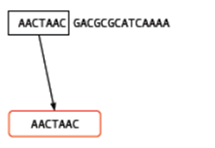
You may well ask, ‘So what? How does that help?’ For a single read, it really doesn’t help. However let’s say that you have another read which is identical except for a single base:

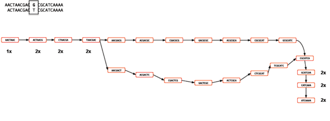
Rather than represent both reads separately, we need only store the k-mers which differ and the number of times they occur. Note the ‘bubble’ like structure which occurs when a single base-change occurs. This kind of representation of reads is called a ‘k-mer graph’ (sometimes inaccurately referred to as a de-bruijn graph).

Now let’s see what happens when we add in a third read. This is identical to the first read except for a change at another location. This results in an extra dead-end being added to the path.

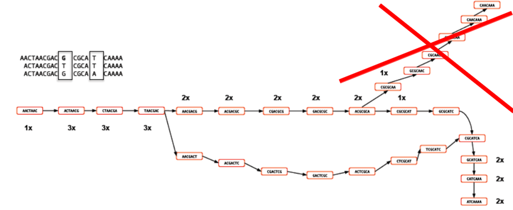
The job of any k-mer based assembler is to find a path through the k-mer graph which correctly represents the genome sequence.

Images courtesy of Mario Caccamo

Description of coverage cutoff:

In the figure above, you can see that the coverage of various k-mers varies between 1x and 3x. The question is which parts of the graph can be trimmed or removed so that we avoid any errors. As the graph stands, we could output three different contigs as there are three possible paths through the graph. However, we might wish to apply a coverage cutoff and remove the top right part of the graph because it has only 1x coverage and is more likely to be an error than a genuine variant.

In a real graph you would have millions of k-mers and thousands of possible paths to deal with. The best way to estimate the coverage cutoff in such cases is to look at the frequency plot of contig (node) coverage, weighted by length. In the example below you can see that contigs with a coverage below 7x or 8x occur very infrequently. As such it is probably a good idea to exclude those contigs which have coverage less than this - they are likely to be errors.

Description of expected coverage:

In the example below you can see a stretch of DNA with many reads mapping to it. There are two repetitive regions A1 and A2 which have identical sequence. If we try to assemble the reads without any knowledge of the true DNA sequence, we will end up with an assembly that is split into two or more contigs rather than one.

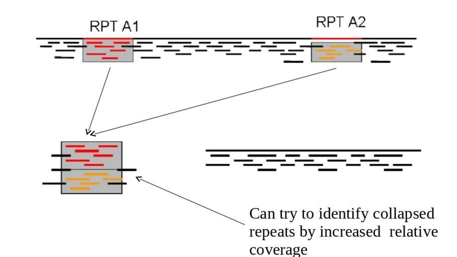
One contig will contain all the reads which did not fall into A1 and A2. The other will contain reads from both A1 and A2. As such the coverage of the repetitive contig will be twice as high as that of the non-repetitive contig.

If we had 5 repeats we would expect 5x more coverage relative to the non-repetitive contig. As such, provided we know what level of coverage we expect for a given set of data, we can use this information to try and resolve the number of repeats we expect.

A commonly used metric to describe the effectiveness of the assembly is called N50 - see http://en.wikipedia.org/wiki/N50_statistic for details.

Task 2: Checking the assembly

Change into the denovo_assembly directory:

cd denovo_assembly

Firstly we can filter out low coverage and very short contigs using a perl script:

filter_low_coverage_contigs.pl < contigs.fasta > contigs.goodcov.fasta

We will use QUAST again (http://quast.sourceforge.net/quast) to generate some statistics on the assembly.

quast.py --output-dir quast contigs.goodcov.fasta

This will create a directory called quast and create some statistics on the assembly you produced.

cat quast/report.txt

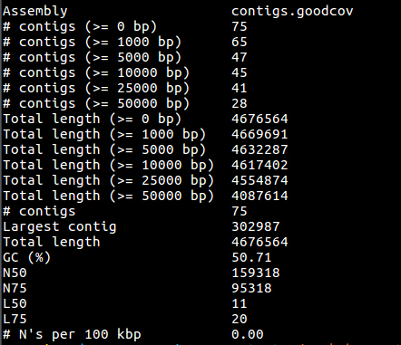
You can see that there are 75 contigs in the assembly - so it is still far from complete. The N50 is 159K and the N75 is 95K so most of the assembly is in quite large contigs. This is fairly normal for a short read assembly - don’t expect complete chromosomes.

Task 3: Map reads back to assembly

A good check at this point is to map the original readsback to the contigs.fasta file and check that all positions are covered by reads. Amazingly it is actually possible for de-novo assemblers to generate contigs to which the original reads will not map.

Here we will use BWA again to index the contigs.fasta file and remap the reads. This is almost identical to the procedure we followed during the alignment section, the only difference is that instead of aligning to the reference genome, we are aligning to our newly created reference.

Make sure you are in the following directory: cd ~/workshop_materials/genomics_tutorial/data/sequencing/ecoli_exeter/denovo_assembly/

Let’s create a subdirectory to keep our work separate

mkdir remapping_to_assembly
cd remapping_to_assembly
cp ../contigs.fasta .

Let’s start by indexing the contigs.fasta file. Type:
bwa index contigs.fasta

Once complete we can start to align the reads back to the contigs. Type (all on one line):

bwa mem -t 2 contigs.fasta ../../E_Coli_CGATGT_L001_R1_001.filtered.fastq ../../E_Coli_CGATGT_L001_R2_001.filtered.fastq > E_Coli_CGATGT_L001_filtered.sam

Once complete we can convert the SAM file to a BAM file:

samtools view -bS E_Coli_CGATGT_L001_filtered.sam > E_Coli_CGATGT_L001_filtered.bam

And then we can sort the BAM file:

samtools sort -o E_Coli_CGATGT_L001_filtered.sorted.bam E_Coli_CGATGT_L001_filtered.bam

Once completed, we can index the BAM file:

samtools index E_Coli_CGATGT_L001_filtered.sorted.bam

We can then (at last!) obtain some basic summary statistics using the samtools flagstat command:

samtools flagstat E_Coli_CGATGT_L001_filtered.sorted.bam

We can see here that very few of the reads do not map back to the contigs. Importantly 98% of reads are properly paired which gives us some indication that there are not too many mis-assemblies.

Run qualimap to get some more detailed information (and some images)

qualimap bamqc -outdir bamqc -bam E_Coli_CGATGT_L001_filtered.sorted.bam

firefox bamqc/qualimapReport.html

In the Chromosome stats section:

The larger of our contigs have a mean coverage of around 50 - which is what we would expect from our original alignment.

There is one contig which has the size of 67128 and much higher coverage - this is exactly the same as the contig we found in the unmapped reads - a good indication that it is a separate sequence (remember we suspected a plasmid) and not integrated into the chromosome.

Let’s double check that by blasting these contigs against the unmapped assembly contigs from part 4:

blastn -subject ../contigs.goodcov.fasta -query ../../unmapped_assembly/spades_assembly/contigs.fasta > check_plasmid.blastn

Open the file in a text editor:

pluma check_plasmid.blastn

and about 30% of the way down the file you should find: (hint use search/find)

Query= NODE_1_length_67364_cov_602.091

Length=67364

Subject= NODE_24_length_67128_cov_604.709

Length=67128


 Score = 1.164e+05 bits (63055),  Expect = 0.0
 Identities = 63057/63058 (99%), Gaps = 0/63058 (0%)
 Strand=Plus/Minus

This shows us that this contig exactly almost matches that in the unmapped assembly, strongly supporting that this is a plasmid sequence and not integrated into the chromosomes.

Task 4: View assembly in IGV Load up IGV
igv.sh

Click Genomes -> Load Genome from File. We are going to import the contigs we have assembled as the reference. Unlike the reference genome though, we have no annotation available. Make sure you select the contigs.goodcov.fasta file for the complete de novo assembly (not the unmapped reads assembly).

Once loaded, click on File->Load From File select the E_Coli_CGATGT_L001_filtered.sorted.bam file. Again, make sure you load the file in the remapping_to_assembly directory.

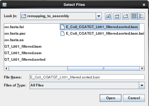
Once loaded, explore some of the contigs in IGV. See if you can find anything unusual in any of the contigs. ** Here is one to get you started - Select NODE_3

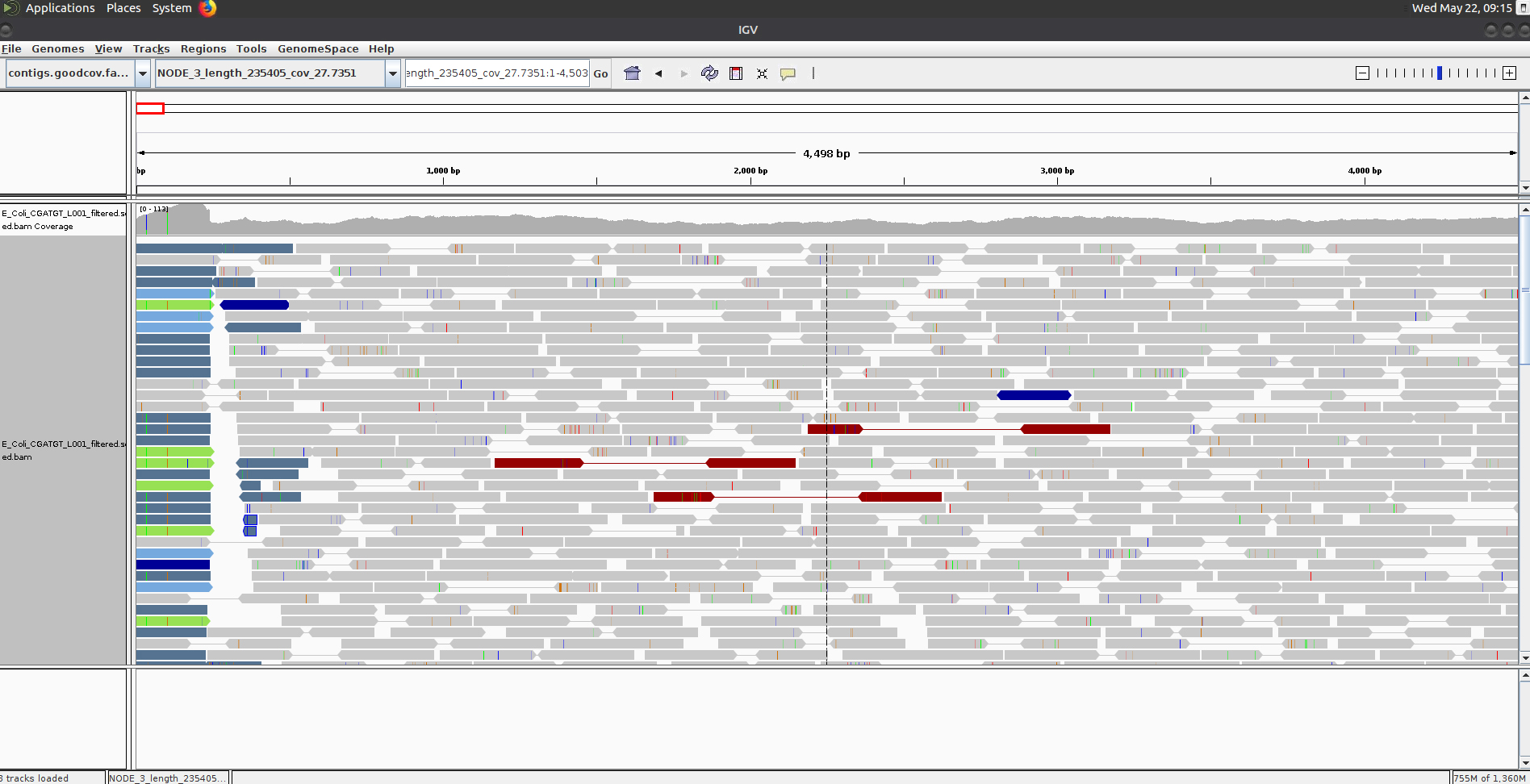
Why does the contig start and end in repetitive sequence (indicated by the coloured / white reads = low mapping quality)? You may need to zoom in to see the details. Think about what an assembler will do if it cannot uniquely assign reads.

If an assembler cannot resolve these repetitive regions with paired-end reads or coverage information, it will generally be unable to assemble any further sequence for that contig. Therefore it is quite common to see contigs which start and end in sequence which is repeated elsewhere.

Here is another - Select NODE_48.

Right click on the reads and select view as pairs:

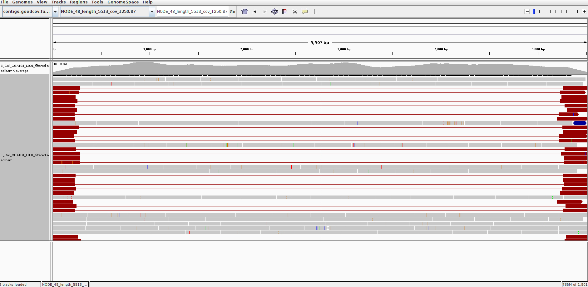
What do you think is going on here? Try blasting the contig sequence using BlastX at http://blast.ncbi.nlm.nih.gov/Blast.cgi to identify which genes the contig contains. To obtain the sequence you can right click and select ‘Copy consensus sequence’

You can also do the same for individual reads, but you need to un-select ‘View as pairs’ before right clicking on a read. You may lose track of the paired-end reads and find it easier to copy the read name before un-selecting ‘View as pairs’ and then and then pasting it into the ‘Select by name’ search box.

You should find that the contig contains at least two phage genes. There appear to be at least two phages present, one which seems to be the full contig, the other with the red read-pairs seems to be missing the sequence in the middle of the contig.

Annotation of de-novo assembled contigs

We will now annotate the contigs using BLAST, Pfam and RAST as with the unmapped contigs.

Task 5: Obtain open reading frames

As before, we’ll call open reading frames within the de-novo assembly. Again, we will use codon table 11 which defines the bacterial codon usage table (http://www.ncbi.nlm.nih.gov/Taxonomy/Utils/wprintgc.cgi) and state that the sequences we are dealing with are not circular. We will also restrict the ORFs to just those sequences longer than 300 nucleotides (i.e. 100 amino acids). We will store the results in file contigs.orf.fasta.

Make sure you are in the denovo_assembly/ directory:

getorf -table 11 -circular N -minsize 300 -sequence contigs.goodcov.fasta -outseq contigs.orf.fasta

The following two tasks are optional. Be warned - the BLAST searches and RAST will take several days! I recommend you start these now and then these and proceed to Task 9.

Task 6 (Optional): Search open reading frames against NCBI non-redundant database

We can also search these open reading frames against the NCBI non-redundant database.

blastp -db ~/workshop_materials/genomics_tutorial/db/blast/nr -query contigs.orf.fasta -evalue 1e-06 -num_threads 4 -show_gis -num_alignments 10 -num_descriptions 10 -out contigs.orf.fasta.blastp

Task 7 (Optional): Search contigs against NCBI non-redundant database

The following command executes a nucleotide BLAST search (blastn) of the sequences in the contigs.fasta file against the non-redundant database. Again we restrict ourselves to 10 results per hit and an e-value cutoff of 1e-06.

blastn -db ~/workshop_materials/genomics_tutorial/db/blast/nt -query contigs.fasta -evalue 1e-06 -num_threads 4 -show_gis -num_alignments 10 -num_descriptions 10 -out contigs.fasta.blastn

Task 8 (Optional) Run the contigs through the RAST server and import the resulting GFF annotation into IGV (refer back to Part 3 for instructions).

Task 9: Run open reading frames through Pfam

As with the unmapped reads we will search the open reading frames against the Pfam HMM database of protein families. Later on we will be able to use these results to identify Pfam domains which are unique to a particular strain.

pfam_scan.pl -fasta contigs.orf.fasta -dir ~/workshop_materials/genomics_tutorial/db/pfam/ -outfile contigs.orf.pfam -cpu 2 -pfamB -as

This will take around 5 hours so it is recommended that you leave this running while continuing with the rest of the tutorial. If it is still running when you finish your session for today, leave your instance running overnight, but please be sure to turn it off in the morning!

Hybrid Assembly

You will have seen that even with good coverage and a relatively long (300bp) paired end Illumina dataset - the assembly we get is still fairly fragmented. Our E.coli example assembles into 75 contigs and the largest contig is around 10% of the genome size.

Why is this?

One possible reason would be that regions of the original genome were not sequenced, or sequenced at too low coverage to assemble correctly. Regions of the genome will occur with different frequencies in the library that was sequenced - You can see this in the variation of coverage when you did the alignment. This can be due to inherent biases in the preparation and the random nature of the process.

However as coverage increases the chances of not sequencing a particular region of the genome reduces and the most significant factor becomes the resolution of repeats within the assembly process. If two regions contain the same or very similar sequences the assembler cannot reliably detect that they are actually two or more distinct sequences and incorrectly ‘collapses’ the repeat into a single sequence. The assembler is now effectively missing a sequence and therefore breaks in the assembly occur.

One resolution to this is to use a sequencing technology like PacBio or Sanger which can produce longer reads - the reads are then long enough to include the repeated sequence, plus some unique sequence, and the problem can be resolved. Unfortunately getting enough coverage using Sanger sequencing is expensive and PacBio - although relatively inexpensive has a high error rate.

An approach becoming more and more popular is to combine technologies. For example: high quality Illumina sequencing to get the accuracy of reads combined with low quality PacBio sequencing to enable the repeats to be spanned and correctly resolved.

Our exercise will be to use Illumina and PacBio datasets to assemble a species of Pseudomonas. These are subsets of data used in “Evaluation and validation of de novo and hybrid assembly techniques to derive high-quality genome sequences” Utturkar et al., 2014. (http://www.ncbi.nlm.nih.gov/pubmed/24930142).

This paper also contains a good explanation of the process and different approaches that are available.

Note our example is not a particularly good dataset and the improvement is quite modest.

Firstly, as always, it is important to check and understand the quality of the data you are working with: Change to the directory and run fastqc

cd ~/workshop_materials/genomics_tutorial/data/sequencing/pseudomonas_gm41
fastqc

Open the files SRR1042836a.fastq SRR491287a_1.fastq and SRR491287a_2.fastq and look at the re- ports generated.

Note that the quality of the PacBio reads (SRR1042836a.fastq) is much lower than the Illumina reads with a greater than 1 chance in 10 of there being a mistake for most reads.

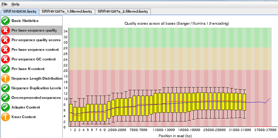
However, importantly, the length of the PacBio reads is much longer.

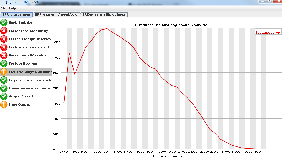
Trim the Illumina reads as before:

fastq-mcf ../../reference/adaptors/adaptors.fasta SRR491287a_1.fastq SRR491287a_2.fastq -o SRR491287a_1.filtered.fastq -o SRR491287a_2.filtered.fastq -q 20 -p 10 -u -x 0.01

You can check the number of filtered reads using grep -c and the quality of trimmed reads with fastqc if you want.

For this exercise we want the long reads from PacBio even though they are low quality. We are relying on the assembler to use them appropriately.

Task 11: Illumina Only Assembly

Firstly let’s construct an assembly using only the available Illumina data. Make sure you are in the directory cd ~/workshop_materials/genomics_tutorial/data/sequencing/pseudomonas_gm41

and Run:

spades.py --threads 2 --careful -o illumina_only_assembly -1 SRR491287a_1.filtered.fastq -2 SRR491287a_2.filtered.fastq

This may take some time so the data has been precomputed and is available in illumina_assembly if you are impatient!

Change to the directory:
cd illumina_only_assembly

Filter out low coverage and very short contigs using a perl script:
filter_low_coverage_contigs.pl < contigs.fasta > contigs.goodcov.fasta

Let’s look at the metrics for the assembly.
quast.py --output-dir quast contigs.goodcov.fasta

cat quast/report.txt

Your results may be slightly different. This is because spades uses a random seed that changes every time

Task 12: Create Hybrid Assembly

Now will execute the same command, but this time include the longer PacBio reads to see the effect it has on our assembly. Change back into the directory
cd ~/workshop_materials/genomics_tutorial/data/sequencing/pseudomonas_gm41

Run (This may take some time so the data has been precomputed and is available in hybrid_assembly_pre/ if you are impatient!):

spades.py --threads 2 --careful -o hybrid_assembly --pacbio SRR1042836a.fastq -1 SRR491287a_1.filtered.fastq -2 SRR491287a_2.filtered.fastq

Change to the directory:
cd hybrid_assembly

Filter out low coverage and very short contigs using the perl script:
filter_low_coverage_contigs.pl < contigs.fasta > contigs.goodcov.fasta

Let’s look at the metrics for the assembly - this time we will compare it with the illumina only assembly:
quast.py --output-dir quast contigs.goodcov.fasta ../illumina_only_assembly/contigs.goodcov.fasta

cat quast/report.txt

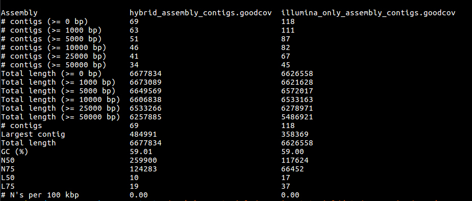
firefox quast/report.html

It seems that using the longer reads has improved the completeness of our assembly - reducing the number of contigs. In truth, this is a very modest improvement, for bacteria it is difficult to find a dataset where the long reads help, without making the short reads redundant and assembling eukaryotes would take too long in the context of the course.

Task 13: Align reads back to reference Let’s realign our original reads back to the assembly and see what we have - refer to previous notes if you are unsure of the steps.

Start in the hybrid assembly directory

cd ~/workshop_materials/genomics_tutorial/data/sequencing/pseudomonas_gm41/hybrid_assembly
mkdir remapping_to_assembly
cd remapping_to_assembly
cp ../contigs.fasta .
bwa index contigs.fasta

bwa mem -t 2 contigs.fasta ../../SRR491287a_1.filtered.fastq ../../SRR491287a_2.filtered.fastq > gm41.illumina.sam
samtools view -bS gm41.illumina.sam > gm41.illumina.bam
samtools sort -o gm41.illumina.sorted.bam gm41.illumina.bam  
samtools index gm41.illumina.sorted.bam
samtools flagstat gm41.illumina.sorted.bam

We can also map the PacBio reads, but we need to tell bwa we are using PacBio reads

bwa mem -t 2 -x pacbio contigs.fasta ../../SRR1042836a.fastq > gm41.pacbio.sam
samtools view -bS gm41.pacbio.sam > gm41.pacbio.bam
samtools sort -o gm41.pacbio.sorted.bam  gm41.pacbio.bam  
samtools index gm41.pacbio.sorted.bam
samtools flagstat gm41.pacbio.sorted.bam

You will notice that not such a high proportion of PacBio reads map back to the assembly.

Now start igv:
igv.sh

Load your assembled genome - Click on genome - load from file

Make sure you get the assembly from the hybrid_assembly (igv remembers the previous directory which may contain similar files.)

Now load your 2 alignment files:
click on load from File and then select gm41.pacbio.sorted.bam and gm41.illumina.sorted.bam

On the toolbar select - “Show Details on Click”

Find a region that has decent coverage of both reads and zoom in. (Region shown here: NODE_43_length_17566_cov_24.3317:8,699-8,867)

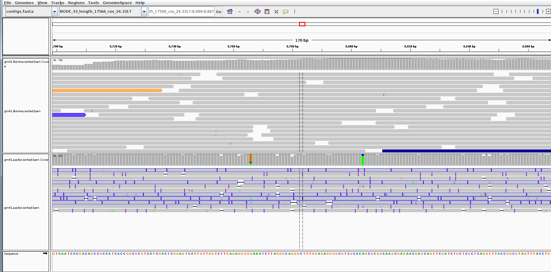
You can see that the PacBio reads are much longer, but the error rate particularly insertions and deletions is much higher than for the Illumina reads.

Explore a few other contigs to see if you can find something that looks like an error or mis-assembly. Remember the assembly process is difficult and far from perfect.

Summary

You have seen that de-novo assembly of short reads is a challenging problem. Even for small genomes, the resulting assembly is fragmented into contigs and far from complete.

Incorporating longer reads to produce a hybrid assembly can be used to reduce the fragmentation of the genome. We have only used a single (perhaps the simplest) technique to incorporate long reads. You can read more about hybrid assembly techniques here: http://www.ncbi.nlm.nih.gov/pubmed/24930142

Part 5. Comparative Analysis

Introduction:

In the previous sections you have been taken through the steps required to:

1. QC and filter Illumina data
2. Remap Illumina short-read data to a reference sequence
3. View the results in IGV
4. Identify SNPs and Indels in an automated fashion using samtools and bcftools
5. Determine whether SNPs result in synonymous or non-synonymous changes in the corresponding amino acid
6. Extract unmapped reads
7. Assemble unmapped reads and obtain assembly statistics
8. Annotate unmapped reads using Pfam, RAST and/or BLAST
9. Assemble a bacterial genome de-novo using SPAdes
10. Obtain assembly statistics
11. Annotate as per the unmapped reads (where computationally feasible).

Now we want you to do the same on a set of Vibrio parahaemolyticus strains which have been isolated and sequenced. There are six strains available depending on how much time is available and enthusiasm you have - choose a number of strains (at least 2) as we want to run some comparisons.

The strains can be found in:

cd ~/workshop_materials/genomics_tutorial/data/sequencing/Vibrio_parahaemolyticus

Under each Sample directory is a subdirectory called raw_illumina_reads which contains the fastq files.

For remapping, the reference can be found in the folder:
~/workshop_materials/genomics_tutorial/data/reference/Vibrio_parahaemolyticus_RIMD_2210633_uid57969 (Remember, you will need to create an index first).

For each strain, make a list of:

• SNPs, Indels and their effects (from the remapping)
• Missing genes (from the remapping)
• Novel plasmids and/or genes (Pfam domains are the easiest way to do this via denovo assembly of unmapped reads - when performing the assembly - don’t specify the k-mers SPAdes will choose appropriate ones.)

Once completed, see if you can predict what the phenotype of these bacteria might be. Then proceed to the final part of the tutorial where we will compare the results from all of these strains.

N.B. It is recommended that you follow the same directory naming convention we have followed here (i.e. one for remapping to the reference, another for assembly of unmapped reads and a final one for the denovo assembly).

These tasks may take you several days. However, remember that all of the basic procedures are detailed in the previous sections - only the input FASTQ files will have changed. Feel free to refer to these previous tasks to remind yourself of the commands and parameters. By all means feel free to play around with different parameters if you wish, although remember that the results may differ from those you see here.

Just to give you some guidance:

You should find that strain Sample_T0347070 yields many more SNPs than other strains.

You may find that some scripts and programs run more slowly because of these extra differences and larger datasets.

Also, if you find the de novo assembly process causes your session to end, the chances are that SPAdes has caused your instance to run out of memory. If this happens, increase the minimum k-mer size in the spades.py command line.

Here we will use a script to compare the variants called in each sample. Ensure you are in the
~/workshop_materials/genomics_tutorial/data/sequencing/Vibrio_parahaemolyticus directory

First of all, let’s make a directory to store the results of the comparison:

mkdir snp_comparison

We need a copy of all of the vcf4 files we created here. This is a quick way to do it - paste this in as one command

for sample in Sample*
do
cp -v $sample/remapping_to_reference/out.snps.vcf4 snp_comparison/\$sample.out.snps.vcf4
done

cd snp_comparison

Note that the copy commands may require modification depending on where you have saved the variant call results.

Our directory contents should look something like:

We’ll now set up some variables so we don’t have to type long path names

ref=~/workshop_materials/genomics_tutorial/data/reference/Vibrio_parahaemolyticus_RIMD_2210633_uid57969/Vibrio_parahaemolyticus_RIMD_2210633_uid57969.fasta

gff=~/workshop_materials/genomics_tutorial/data/reference/Vibrio_parahaemolyticus_RIMD_2210633_uid57969/Vibrio_parahaemolyticus_RIMD_2210633_uid57969.gff

samples=`ls *.vcf`

We can now use $ref instead of the long path to our reference and $gff for the feature file. e.g.

head $ref
echo $samples

When we are happy our variables are correct then run:

snp_comparator.pl 10 $ref $gff $samples > snp_comparison.txt

Looking at the snp_comparison.txt file (either in a text editor, or in a spreadsheet):
If you have chosen different samples - you will get different results of course.

Here we can see the chromosome ID, the position in bp, the reference base and the base at each position as well as the gene (if any) the variant occurs in as well as the effect (silent, non-silent or indel).

Obtaining a phylogeny based on synonymous SNPs only:

How are the strains related on the basis of these variants? We can ask a number of questions, but if we are looking at the long-term evolutionary history of the strains we should only look at synonymous (i.e. silent) mutations as these should not confer a significant selective advantage to any strain. Using the data snp_comparison.txt file, we can form ‘pseudo-sequences’ using the script snp2tree_fullsequence.pl

These are concatenated bases consisting of only those positions which are silent across all strains. It is essentially the same as turning each column of each strain in the snp_comparison.txt file into a FASTA entry.

snp2tree_fullsequence.pl snp_comparison.txt > synonymous_tree.fasta

Examine the contents of the tree.fasta file. We can then treat this file as an alignment (since each base in each sequence is at the same position on the chromosome) and pass it to a phylogeny program called FastTree. FastTree will take an input alignment and output a Newick formatted tree (http://en.wikipedia.org/wiki/Newick_format). \

FastTree -nt -gtr < synonymous_tree.fasta > synonymous_tree.newick

Now we can visually view this tree by using an online tool.

firefox http://www.trex.uqam.ca/index.php?action=newick

Either paste the contents of the .newick file into the window or select ‘Sequences file’ and load the file through the browser. Then select ‘View Tree’

Advanced task:

Copy the snp2tree_fullsequence.pl script to this directory: (~/workshop_materials/genomics_tutorial/data/sequencing/Vibrio_parahaemolyticus/snp_comparison) and modify it so that it selects positions containing only non-silent mutations (not indels as these modify the alignment). Generate a new alignment and compare the resulting tree against the silent mutations.

You will need to have some experience of programming in the Perl language to do this.

Part 6. Long Read Assembly

Introduction:

The latest third-generation sequencing platforms from Oxford Nanopore and Pacific Biosciences enable sequencing of single DNA molecules. Remember second generation sequencing platforms (e.g. Illumina) rely on sequencing a group of ~1000 mono-clonal molecules formed via PCR-like reactions. This has advantages in terms of reducing the quantity of DNA input required to enable sequencing, usually enables lower per-base costs, but has many shortcomings.

In the case of Illumina, although the sequencer is capable of generating large quantities of data (terabases in the case of a HiSeq run), the amplification step introduces GC-biases and also places a maximum limit on the size of the fragments which can be sequenced since the amplification becomes inefficient at larger fragments sizes and sequencing becomes de-phased within individual mono-clonal clusters due to polymerase errors. In the case of genome assembly, this introduces fragmentation of the assembly in areas of low coverage or repetitive regions which cannot be spanned.

Third generation sequencing of single molecules has the following features:

• Ability to sequence native genomic DNA without limitations on size (100s kilobases are possible)
• Higher single pass per-base error rates than second-generation sequencers
• Higher per-base cost than second-generation sequencing
• Full length cDNA or amplicon sequencing
• Some platforms such as the MinION from Oxford Nanopore hold the potential to enable portable sequencing and sequencing of other types of nucleic acid (e.g. RNA).

PacBio sequencing

You can watch a video outlining PacBio sequencing at http://sequencing.exeter.ac.uk/pacific- biosciences-overview/.

Pacific Biosciences have two sequencing platforms - RSII and Sequel. The RSII is an older platform capable of generating around 750Mbases of data in 4-6 hours. The Sequel platform is the latest platform and in theory can generate up to 7G bases of data in a similar time frame. However the chemistry is still being refined and at present 4-5 Gbases is the maximum which should be expected.

The Sequel platform is PacBio’s focus for development at the moment, with optics included on the chip rather than the instrument, PacBio aims to increase the number of Zero Mode Waveguides (ZMWs) to increase throughput without significant instrument modifications.

PacBio SMRTcells (RSII left - Sequel right)

PacBio Yield and read length distributions (RSII left - Sequel right)

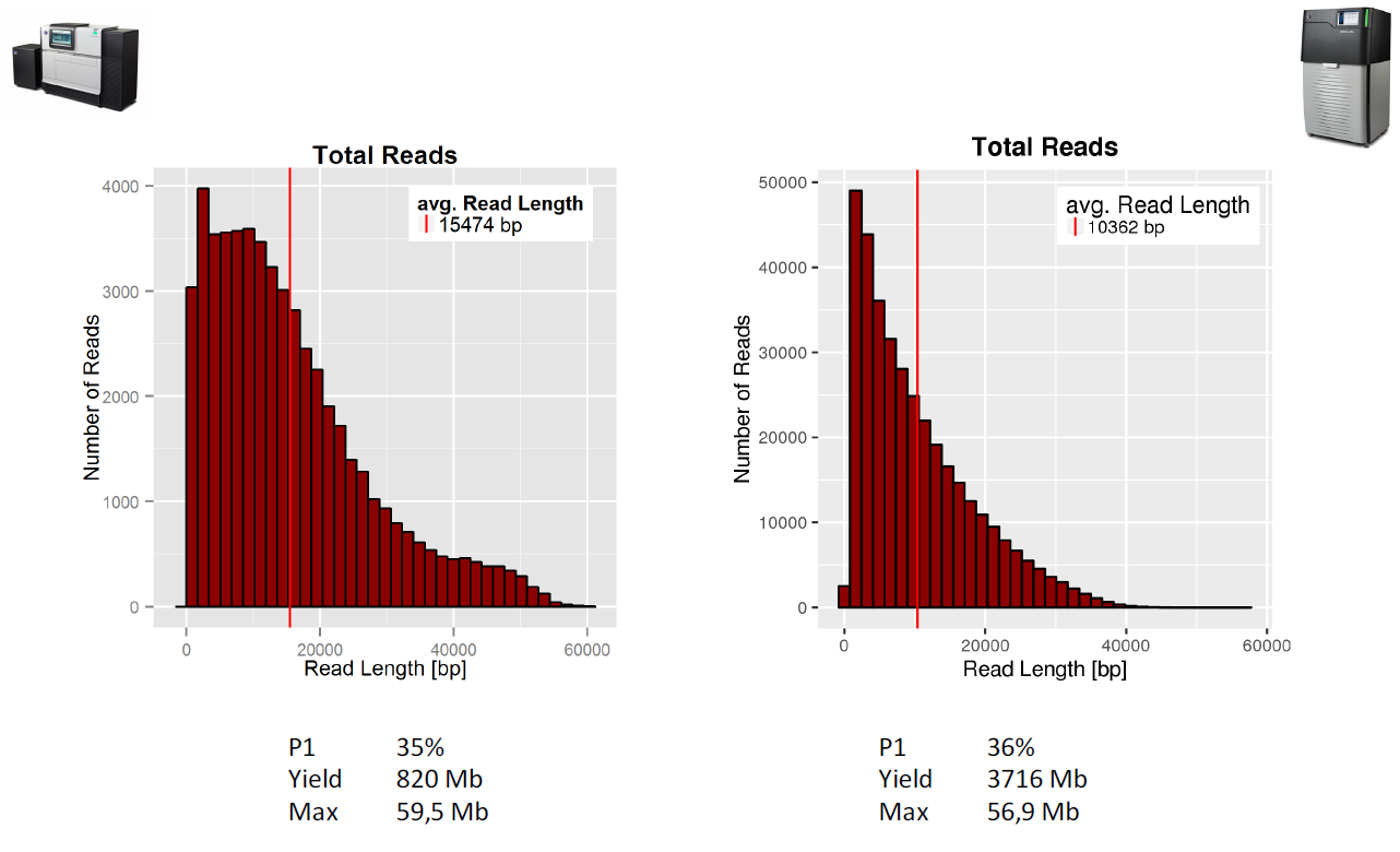
A typical genomic library preparation workflow is similar to that of Illumina sequencing with the difference that much higher molecular weight DNA is used and dumb-bell shaped adaptors are attached:

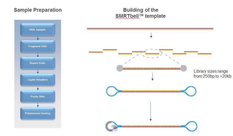
An important note regarding PacBio data quality

PacBio libraries are circular. Because of this, a single polymerase can sequence the same piece of DNA several times. However, a balance exists between the DNA template length, polymerase life time (also known as polymerase read length) and read quality with PacBio data. The figure below illustrates this.

A polymerase which is able to read for 10kb, could read a single 10kb template or, for example, it could read a 2kb template 5 times. The 2kb fragment, having been read 5 times, would be of much higher quality than the 10kb fragment.

Terminology which is important to understand with PacBio data is highlighted in above. A polymerase read refers to the complete set of basecalls associated with the polymerase sequencing the forward strand, adaptor, and reverse strand. Internally, we remove the adaptor sequences and provide the subreads (just the forward and reverse sequences of the template). These can be further analysed to produce circular consensus reads (CCS) if the enzyme has made more than 1 pass of the molecule.

Most assembly programs require the subreads if utilizing PacBio data.

MinION sequencing technology:

This is a radically new sequencing technology based upon monitoring electrical current fluctuations associated with the translocation of single DNA molecules through nanopores embedded in a membrane. You can read more about the technology in detail https://nanoporetech.com/how-it-works

This is a remarkable technology which has the potential to supplant short-read sequencing, if the error rates can be brought down sufficiently. It has the advantage of being portable and of generating long fragment lengths.

A typical long read assembly pipeline:

• Generate and evaluate QC metrics
• Perform an initial assembly with Minimap/Miniasm to check whether we have sufficient data
• Check for any potential contamination in the Miniasm assemblies using Blast and Krona
• Correct long reads via consensus alignment and assemble
• Polish the assembly with Illumina or other short-read data
• If necessary, attempt to circularize the genome correctly
• Compare assemblies against the reference using Quast
• Generate gene predictions and/or functional annotation

We have provided you with data generated from the same strain of E.coli K12 MG1655 across three different platforms - Oxford Nanopore MinION, PacBio RSII and PacBio Sequel. The MinION data was generated and published by Nick Loman and Josh Quick whilst the PacBio data was generated at Exeter from the same material.

We have provided you with data from both 1D and 2D libraries. Remember these are two different types of library preparation. A 1D library enables just the template strand of the DNA molecule to be read, whilst a 2D library enables both the template and complement strand to be sequenced. This means that a 2D library will be sequenced. (Recently 1D squared has replaced the 2D libraries)

The datasets can be found in the directory:

~/genomics_tutorial/long_read_tutorial/raw_data

Note that we have four datasets in total - Sequel, RSII, MinION 1D and MinION 2D the MinIon dataset consists of two fasta files. One is a 1D dataset and another is a 2D dataset. Note that typically MinION datasets are generated in a binary formatted file on a per-read basis which contain the current-levels and other data. However, for simplicity we have converted these into fasta files.

We’ll follow a similar analysis protocol for all 4 datasets (some are pre-generated).

Task 1 Generate basic statistics for each of these datasets

You can use the fasta_summary.pl script to do this for both fasta-formatted MinION datasets. It might take a while to compute, therefore we have pre-computed the results for you:

fasta_summary.pl -i E_coli_K12_1D_R9.2.pass.fasta -o E_coli_K12_1D_summary -t read

fasta_summary.pl -i E_coli_K12_2D_R9.0.pass.fasta -o E_coli_K12_2D_summary -t read

~/workshop_materials/genomics_tutorial/long_read_tutorial/pre_computed_results/canu_assemblies/fasta_summaries

For the PacBio data you can use the fastqc program as per the Illumina datasets you have looked at previously.

The fasta_summary.pl script will generate several output files:

• stats.txt file contains text-data on the number of bases, longest read and other useful statistics.
• histograms_bins.dat.png file is a picture file with a histogram of read lengths (you can use firefox to see the file).

Task 2: Compare the datasets

Note that unlike Illumina sequencers, the read lengths produced by these platforms are highly variable. The MinION datasets for example vary between 100bp and 140,000bp.

Note the relatively poor quality scores in the fastqc report for the PacBio sequences. These reflect the 10-12% raw single-pass per-base error rate of the polymerase. Similar error rates are observed in the MinION datasets. Note that unlike Illumina datasets, this error rate does not appreciably increase over the length of the read (although at very short or very long read lengths there are far fewer reads present which increase the variance estimates).

Task 3: Evaluate the likelihood of obtaining a successful assembly using Minimap/Miniasm

This very useful assembler tries to assemble long-reads without trying to correct the reads. Although you would not want to use such an assembly without further correction, it provides a useful yardstick to determine whether a more computationally intensive assembly is likely to yield good results. You can read more here https://github.com/lh3/miniasm.

Because of limitations on the memory available to us, we’ll need to subset the data first, selecting a random 100,000 reads to use (note that this is not the best approach since we should really pick the longest 100,000 reads).

The syntax can be a bit confusing, so here is an example using the RSII dataset to get you started. Each assembly should take about 5-10 mins.

Create a new working directory in ~/workshop_materials/genomics_tutorial/long_read_tutorial called miniasm_assemblies

cd ~/workshop_materials/long_read_tutorial
mkdir miniasm_assemblies

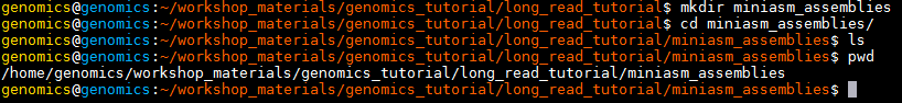
We’ll use the seqtk package from the same author as samtools to randomly select 100,000 reads from the raw dataset:

seqtk sample ~/workshop_materials/genomics_tutorial/long_read_tutorial/raw_data/RSII_Ecoli_K12_subreads.fastq 100000 > RSII_Ecoli_K12_subreads.subsampled.fastq

Now we can ask minimap to calculate all the overlaps between those 100,000 reads and output the results in a compressed gzip file. Note that you will have to put the input reads (RSII_Ecoli_K12_subreads.subsampled.fastq) in twice - since we are asking minimap to calculate the overlaps between all reads in the dataset:

minimap -Sw5 -L100 -m0 -t 2 RSII_Ecoli_K12_subreads.subsampled.fastq RSII_Ecoli_K12_subreads.subsampled.fastq | gzip -1 > overlaps_RSII.paf.gz

Once complete, we can ask miniasm to create an assembly graph and find an assembly path through it:

miniasm -f RSII_Ecoli_K12_subreads.fastq overlaps_RSII.paf.gz > overlaps_RSII.gfa

awk '/^S/{print "\>"\$2"\\n"\$3}' overlaps_RSII.gfa | fold > miniasm.PacBio_RSII.contigs.fasta

Repeat this for the Sequel and MinION datasets and then use the QUAST package (quast.py) to compare the assemblies against the reference genome. You should use the same E.coli reference as you used for the Illumina assemblies.

You should be able to open the report.html file in firefox or other web-browser to compare the assemblies. It should look somewhat similar to:

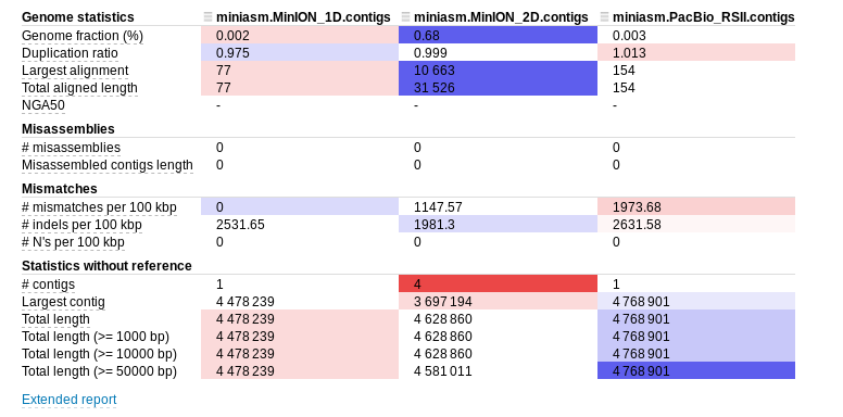
Note that your results will differ since you will have a different subset of reads. Minimap/miniasm does not correct reads prior to assembly. This means that the alignments to the reference are likely to be error prone. Note that even without this correction, the assembler is able to reconstruct the genome in (more or less) a single contig of 4.7Mb with just 100,000 reads! This bodes well for a more computationally intensive assembly which first corrects reads and highlights the power of long reads for de-novo assembly.

If you wish you can subset the data with the seqtk sample and compare how the datasets assemble at different levels of coverage.

Task 4: Generate a corrected assembly with Canu (results pre-computed)

Canu is derived from the original Celera assembler used to assemble the human genome from Sanger data. It has been optimized for long-read PacBio and Nanopore data. You can read more at http://canu.readthedocs.io/en/stable/tutorial.html. A number of long read assemblers are available (including Nanopore-specific assemblers - a good review paper on this is:

Chu J, Mohamadi H, Warren RL, Yang C, Bi-Rol I. Innovations and challenges in detecting long read overlaps: an evaluation of the state-of- the-art. Bioinformatics. 2016

For now we will just use Canu as it is relatively straightforward to use. Here is an example command to assemble the RSII E.coli data. We have pre-computed the results for you for the MinION 2D, RSII and Sequel data.

~/workshop_materials/genomics_tutorial/long_read_tutorial/pre_computed_results/canu_assemblies

To save time, and provide a fairer comparison between platforms we will not use the MinION 1D data.

canu -p canu_RSII -d canu_RSII genomeSize=4.7m useGrid=False -pacbio-raw RSII_Ecoli_K12_subreads.fastq

Note that Canu will:

• Correct reads by performing all-against-all alignments and taking a consensus
• Overlap and trim reads
• Generate an assembly

Task 5: Polish Canu assemblies with Illumina data using Pilon (results pre-computed)

Oxford Nanopore and MinION data suffer a tendency to introduce insertions or deletions into a sequence (even after read correction). This means that to obtain the highest per-base quality it is desirable to polish assemblies by aligning short reads using BWA and then using a tool such as Pilon (https://github.com/broadinstitute/pilon/wiki) to polish the assemblies.

We have supplied you with pre-computed results. We’ll use just the RSII data to illustrate an example set of commands. First let’s align the Illumina reads from the short-read section of the workshop using BWA.

We need to create a reference for the PacBio RSII contigs:

bwa index RSII_canu_contigs.fasta

Now we need to align the Illumina reads against the contigs:

bwa mem -x pacbio -t 2 RSII_canu_contigs.fasta ../../../data/sequencing/ecoli_exeter/E_Coli_CGATGT_L001_R1_001.fastq ../.
./../data/sequencing/ecoli_exeter/E_Coli_CGATGT_L001_R2_001.fastq   |   samtools sort -@ 2 -O
bam -o RSII_canu_contigs_illumina_aligned.bam

samtools index RSII_canu_contigs_illumina_aligned.bam

Now that we have aligned the Illumina data against the contigs we can run Pilon to correct the contigs where they differ from the Illumina reads.

pilon --genome RSII_canu_contigs.fasta --frags RSII_canu_contigs_illumina_aligned.bam --changes --outdir RSII_canu_pilon_polished

You can view the corrected contigs in RSII_canu_pilon_polished/pilon.fasta and the see a list of the changes which have been made in RSII_canu_pilon_polished/pilon.changes. Note that most changes correct indels and the much higher number of corrections made for the MinION assembly vs the PacBio assemblies (46558 for MinION 2D vs 387 for RSII and 2247 for Sequel).

We need to interpret these polished results with care. Remember we are using Illumina sequencing which contains all sorts of biases of its own thanks to amplification biases introduced by PCR and other artefacts. As such whilst we might be correcting some errors, we could be introducing Illumina biases into these assemblies. We’re also using Illumina reads which are not quite identical to the reference or the PacBio material which is also not ideal (but often the case in the real world!). We’ll see the effect of this in the final task.

Task 6: Use Blast and Krona to confirm species present in the assembly (results pre- computed)

We can use BLAST to identify taxonomic hits to ensure that we have the correct species present and filter out any contigs resulting from control spike-in DNA or other contaminants. You can also use other tools to do this such as Kraken or Centrifuge.

As the blast searches take some time, the results have been pre-computed for you in

~/workshop_materials/genomics_tutorial/long_read_tutorial/pre_computed_results/krona_plot/

but we have included the commands used below:

blastn -db ../../../db/blast/nt -query RSII_canu_pilon_polished.fasta  -outfmt 7 -evalue 1e-06 -out RSII_canu_pilon_polished.fasta.blastn.outfmt7 -num_threads 2

Once this has completed, we can import the results into Krona which is a neat little visualization tool for BLAST results. ** ktImportBLAST -i RSII_canu_pilon_polished.fasta.blastn.outfmt7 -o krona_blast_results.html

These results can be visualized in a web-browser such as firefox.

Note that the MinION data contains Lambda virus DNA which is used as a spike-in to some MinION runs. You can identify which contigs hit species of interest by clicking on the area of the pie chart you are interested in and then clicking on the ‘Count’ in the top right corner. This wil give you the contig names which match to the virus as opposed to the bacteria.

Task 7: Circularise assemblies using Circlator (results pre-computed)

Note that bacterial genomes are circular. As such we may end up mis-assembling the genome because it is circular. The circlator package (https://github.com/sanger/pathogens/circlator/wiki/Minimus2-circularization-pipeline) attempts to correct this.

In the circularized_results directory you will find the results of the circularization pipeline.

Task 8: Compare polished assemblies using Quast

Use quast.py to generate a report for the original Canu results (i.e. pre Illumina correction and circularization) and these corrected and circularized results. E.g (all on one line):

quast.py -R ~/workshop_materials/genomics_tutorial/data/reference/U00096/U00096.fna MinION_2D_canu_pilon_polished.circularise.fasta
~/workshop_materials/genomics_tutorial/long_read_tutorial/pre_computed_results/canu_assemblies/MinION_2D.contigs.fasta RSII_canu_pilon_polished_circularise.fasta ~/workshop_materials/genomics_tutorial/long_read_tutorial/pre_computed_results/canu_assemblies/
RSII_canu_contigs.fasta Sequel_canu_pilon_polished.circularise.fasta
~/workshop_materials/genomics_tutorial/long_read_tutorial/pre_computed_results/canu_assemblies/Sequel_canu_contigs.fasta

Look at the effect of the polishing step for each technology. Have a think about the following:

• The PacBio reads have a higher mismatch error after polishing but a lower indel rate? (think about the possible effects of PCR amplification on GC-bias)
• What about the total number of contigs for each platform?
• How does the mis-match rate to the reference genome compare between the MinION and the PacBio platforms?
• The Sequel platform used very early chemistry - how does it perform compared to the other platforms?
• Which platform would you select if you wanted to use the assembly as a reference to perform variant calling against?

Concluding remarks:

Well done! If you have reached this far, you deserve a round of applause. You have completed some of the most common tasks in genomics. You can use the same machine and the same scripts to perform analysis of any dataset! If you need to transfer data to/from the instance a tutorial can be found at http://www.siteground.com/tutorials/ssh/ssh_winscp.htm